Download
1 / 46
490 likes | 958 Views
Cost Minimization and Cost Curves. Beattie, Taylor, and Watts Sections: 3.1a, 3.2a-b, 4.1. Agenda. The Cost Function and General Cost Minimization Cost Minimization with One Variable Input Deriving the Average Cost and Marginal Cost for One Input and One Output

E N D
Cost Minimization and Cost Curves Beattie, Taylor, and Watts Sections: 3.1a, 3.2a-b, 4.1
Agenda • The Cost Function and General Cost Minimization • Cost Minimization with One Variable Input • Deriving the Average Cost and Marginal Cost for One Input and One Output • Cost Minimization with Two Variable Inputs
Cost Function • A cost function is a function that maps a set of inputs into a cost. • In the short-run, the cost function incorporates both fixed and variable costs. • In the long-run, all costs are considered variable.
Cost Function Cont. • The cost function can be represented as the following: • C = c(x1, x2, …,xn)= w1*x1 + w2*x2 + … + wn*xn • Where wi is the price of input i, xi, for i = 1, 2, …, n • Where C is some level of cost and c(•) is a function
Cost Function Cont. • When there are fixed costs, the cost function can be represented as the following: • C = c(x1, x2| x3, …,xn)= w1*x1 + w2*x2 + TFC • Where wi is the price of the variable input i, xi, for i = 1 and 2 • Where wi is the price of the fixed input i, xi, for i = 3, 4, …, n • Where TFC = w3*x3 + … + wn*xn • When inputs are fixed, they can be lumped into one value which we usually denote as TFC • Where C is some level of cost and c(•) is a function
Cost Function Cont. • Suppose we have the following cost function: • C = c(x1, x2, x3)= 5*x1 + 9*x2 + 14*x3 • If x3 was held constant at 4, then the cost function can be written as: • C = c(x1, x2| 4)= 5*x1 + 9*x2 + 56 • Where TFC in this case is 56
Cost Function Cont. • The cost function is usually meaningless unless you have some constraint that bounds it, i.e., minimum costs occur when all the inputs are equal to zero. • There are two major uses of the cost function: • To minimize cost given a certain output level. • To maximize output given a certain cost.
Standard Cost Minimization Model • Assume that the general production function can be represented as y = f(x1, x2, …, xn).
Cost Minimization with One Variable Input • Assume that we have one variable input (x) which costs w. Let TFC be the total fixed costs. • Assume that the general production function can be represented as y = f(x).
Cost Minimization with One Variable Input Cont. • In the one input, one output world, the solution to the minimization problem is trivial. • By selecting a particular output y, you are dictating the level of input x. • The key is to choose the most efficient input to obtain the output.
Example of Cost Minimization • Suppose that you have the following production function: • y = f(x) = 6x - x2 • You also know that the price of the input is $10 and the total fixed cost is 45.
Example of Cost Minimization Cont. • Since there is only one input and one output, the problem can be solved by finding the most efficient input level to obtain the output.
Example of Cost Minimization Cont. • Given the previous, we must decide whether to use the positive or negative sign. • This is where economic intuition comes in. • The one that makes economic sense is the following:
Cost Function and Cost Curves • There are many tools that can be used to understand the cost function: • Average Variable Cost (AVC) • Average Fixed Cost (AFC) • Average Cost (ATC) • Marginal Cost (MC)
Average Variable Cost • Average variable cost is defined as the cost function without the fixed costs divided by the output function.
Average Fixed Cost • Average fixed cost is defined as the cost function without the variable costs divided by the output function.
Average Total Cost • Average total cost is defined as the cost function divided by the output function. • It is also the summation of the average fixed cost and average variable cost.
Marginal Cost • Marginal cost is defined as the derivative of the cost function with respect to the output. • To obtain MC, you must substitute the production function into the cost function and differentiate with respect to output.
Example of Finding Marginal Cost • Using the production function y = f(x) = 6x - x2, and a price of 10, find the MC by differentiating with respect to y. • To solve this problem, you need to solve the production function for x and plug it into the cost function. • This gives you a cost function that is a function of y.
Notes on Costs • MC will meet AVC and ATC from below at the corresponding minimum point of each. • Why? • As output increases AFC goes to zero. • As output increases, AVC and ATC get closer to each other.
Production and Cost Relationships Summary • Cost curves are derived from the physical production process. • The two major relationships between the cost curves and the production curves: • AVC = w/APP • MC = w/MPP
Product Curve Relationships • When MPP>APP, APP is increasing. • This implies that when MC<AVC, then AVC is decreasing. • When MPP=APP, APP is at a maximum. • This implies that when MC=AVC, then AVC is at a minimum. • When MPP<APP, APP is decreasing. • This implies that when MC>AVC, then AVC is increasing.
Example of Examining the Relationship Between MC and AVC • Given that the production function y = f(x) = 6x - x2, and a price of 10, find the input(s) where AVC is greater than, equal to, and less than MC. • To solve this, examine the following situations: • AVC = MC • AVC > MC • AVC < MC
Example of Examining the Relationship Between MC and AVC Cont.
Example of Examining the Relationship Between MC and AVC Cont.
Example of Examining the Relationship Between MC and AVC Cont.
Review of the Iso-Cost Line • The iso-cost line is a graphical representation of the cost function with two inputs where the total cost C is held to some fixed level. • C = c(x1,x2)=w1x1 + w2x2
Example of Iso-Cost Line • Suppose you had $1000 to spend on the production of lettuce. • To produce lettuce, you need two inputs labor and machinery. • Labor costs you $10 per unit, while machinery costs $100 per unit.
Example of Iso-Cost Line Cont. • Given the information above we have the following cost function: • C = c(labor, machinery) = $10*labor + $100*machinery • 1000 = 10*x1 + 100*x2 • Where C = 1000, x1 = labor, x2 = machinery
Example of Iso-Cost Line Graphically x2 X2 = 10 – (1/10)*x1 10 x1 100
Notes on Iso-Cost Line • As you increase C, you shift the iso-cost line parallel out. • As you change one of the costs of an input, the iso-cost line rotates.
Input Use Selection • There are two ways of examining how to select the amount of each input used in production. • Maximize output given a certain cost constraint • Minimize cost given a fixed level of output • Both give the same input selection rule.
Cost Minimization with Two Variable Inputs • Assume that we have two variable inputs (x1 and x2) which cost respectively w1 and w2. We have a total fixed cost of TFC. • Assume that the general production function can be represented as y = f(x1,x2).
First Order Conditions for the Cost Minimization Problem with Two Inputs
Implication of MRTS = Slope of Iso-Cost Line • Slope of iso-cost line = -w1/w2, where w2 is the cost of input 2 and w1 is cost of input 1. • MRTS = -MPPx1/MPPx2 • This implies MPPx1/MPPx2 = w1/w2 • Which implies MPPx1 /w1 = MPPx2/w2 • This means that the MPP of input 1 per dollar spent on input 1 should equal MPP of input 2 per dollar spent on input 2.
Example 1 of Cost Minimization with Two Variable Inputs • Suppose you have the following production function: • y = f(x1,x2) = 10x1½ x2½ • Suppose the price of input 1 is $1 and the price of input 2 is $4. Also suppose that TFC = 100. • What is the optimal amount of input 1 and 2 if you want to produce 20 units.
Example 1 of Cost Minimization with Two Variable Inputs Cont. • Summary of what is known: • w1 = 1, w2 = 4, TFC = 100 • y = 10x1½ x2½ • y = 20
Example 1 of Cost Minimization with Two Variable Inputs Cont.
Solving Example 1 Using Ratio of MPP’s Equals Absolute Value of the Slope of the Cost Function
Solving Example 1 Using MRTS from the Isoquant and Setting it Equal to the Slope of the Cost Function
Final Note on Input Selection • It does not matter whether you are trying to maximize output given a fixed cost level or minimizing a cost given a fixed output level, you want to have the iso-cost line tangent to the isoquant. • This implies that you will set the absolute value of MRTS equal to the absolute value of the slope of the iso-cost line.