Download
1 / 21
210 likes | 315 Views
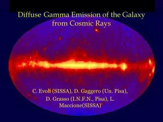
Diffuse Gamma Emission of the Galaxy from Cosmic Rays. C. Evoli (SISSA), D. Gaggero (Un. Pisa), D. Grasso (I.N.F.N., Pisa), L. Maccione(SISSA). EGRET observation. Hunter et al. ‘97. 0 shoulder. Above the GeV a large fraction must be originated by hadronic processes, mainly.

E N D
Diffuse Gamma Emission of the Galaxy from Cosmic Rays C. Evoli (SISSA), D. Gaggero (Un. Pisa), D. Grasso (I.N.F.N., Pisa), L. Maccione(SISSA)
EGRET observation Hunter et al. ‘97 0 shoulder Above the GeV a large fraction must be originated by hadronic processes, mainly Point-sources subtracted p + pgas p + p +0 + ( p + pgas p + p + ± ± + e±+ + e )
How the -ray spectrum extends at high energies ? We expect the -rayspectrum to continue well above 100 GeV It is unknown, however, which fraction is due to hadrons and how that changes across the sky Predictions are still quite model dependent due to poorly known astrophysical parameters Strong et al. ‘04 [GALPROP] 0 decay IC optimized conventional 100 TeV
High energy observatories GLAST Emax ~ 300 GeV Atmospheric Cherenkov Telescopes (HESS, MAGIC, Whipple.. ) 0.1 < E < 100 TeV (best suited for localised sources) MILAGRO Air Shower Arrays (MILAGRO, TIBET AS Gamma) 1 < E < 100 TeV Neutrino Telescopes (ICECUBE,ANTARES,NESTOR,NEMO…) E > 1 TeV May help to solve the hadronic-leptonic origin degeneracy
Our work We focused on the hadronic emission trying to map it as better as possible This component is less (even if not completely) sensitive to local effects We paid attention to: • the CR source (SNR) distribution; • the Galactic Magnetic Fields and their effects on CR diffusion; • the gas distribution and tried to estimate how the uncertainties in the knowledge of those quantities may affect the expected -ray and fluxes
1. SNR distribution Until few years ago SNR (radio shells) survey were used (Case & Bhattacharya ‘96,‘98) (problems: incomplete; selection effects; do not fit radioactive nuclides distr. , e.g. 26Al) SNR are better traced by pulsars and old stars (see Ferriere’01, Lorimer ‘04) Ferriere’01accounts also for SNR not giving rise to pulsars. The peaked distribution exacerbate the problem of reproducing the relatively smooth EGRET flux profile along the GP (see also Strong at al. 2004) “CR gradient problem” Most of the times an “ad hoc” source distribution was chosen to reproduce -rays observations. We adopt Ferriere’s distribution.
2. CR diffusion in the Galactic Magnetic Field(s) zh ~ 1.5 kpc The GMF is a superposition of regular and random fields of comparable strength. By assuming axial symmetry zt ≥ 3 kpc 1 (strong turbulence)Lmax ~ 100 pc << rL (Breg) Propagation takes place in the spatial diffuse regime Most likely turbulence is driven by CR (r) may be higher in SNR rich regions diffusion coefficients may also be spatial dependent Rather than taking a uniform D(E)as estimated from secondary/primary species (e.g. B/C ) we adopt D(E; Breg, ) as derived from MC simulations of particle propagation in turbulent MFs . We adopt exp. from Candia & Roulet 2004 Erlykin & Wolfandale ‘02 considered a spatial dependent turbulent spectrum
CR distribution Diffusion eq. is solved with boundary conditions N(r = 30 kpc, z = zt ) = 0 See e.g. Ptuskin et al. 1993 protons Simulated fluxes are normalized to the observed values (Horandel 2003) at (r,0) Injection spectral slope is tuned to reproduce that observed for protons = 2.7 Inhomogeneous turbulence helps smoothing the CR distribution !
3. Gas distribution H2 is the main target along the Galactic plane. That is generally traced by 12CO (J = 1-0) Dame et al. 2001 The Doppler shift (velocity) + Galaxy rotation curves are used to model the 3-D structure 2-D profiles: Our reference model Nakanishi & Sofue’06 Brofnman et al. ‘88 (corrected) Ferriere et al.’07 We also accounted for HI as determined from 21cm surveys Nakanishi & Sofue’03 Wolfire et al. ‘03 and ref.s therein
Wco models /observations D. Gaggero, thesis work Dame et al. ‘01 (W_CO maps) Nakanishi & Sofue’06 Ferriere et al. ‘07 + Bronfman et al. ‘88 (our work)
XCO The scaling factor XCO = NH2 / WCOis required to convert CO maps into gas column density It is expected to change with r through its dependence on themetallicity That is also required to smooth the -ray profile to make it compatible with the peaked SNR distribution Strong et al. 2004, A&A 422 Strong et al. ‘04 Strong & Mattox ‘96 Our work There is a factor ~ 2 uncertainty. In the inner Galaxy XCO may be lower than what we assumed
Mapping the -ray and emissions (as well as its 3-D generalization) where = 2.7 (proton power law index) ; fN 1.4 accounts for the contribution of other nuclear species in the CR and in the ISM (mainly helium assumed to be distributed like hydrogen nuclei); s is the distance from the observer. Photon and neutrino yields (determined with PYTHIA ( oscillations are accounted for): Y (2.7) = 0.036Y (2.7) = 0.012 Uncertainty ~ 20 % Cavasinni, D.G. and Maccione ‘06; Evoli, D.G. and Maccione ‘07
Comparison with EGRET map ( 4 < E < 10 GeV ) Performed by using a 3-D gas distribution C. Evoli, D. Gaggero, D.G. and L.Maccione, in progress model 2 ( turbulence strength tracing SNRs; Kolmogorov) |l| < 100o |b| < 1o The longitude profile is reasonably reproduced without tuning XCO(r ) and the SNR profile ! The adoption of a more realistic XCO(r ) should allow to improve our fit and leave room for a no negligible IC contribution which is also required to match the latitude profile measured by EGRET (see also Strong at al. 2004)
Expected flux profiles above the TeV C. Evoli, D.G. and L.Maccione, ‘07 CR models 0-3 model 3 uniform CR Berezinsky et al.’93
Comparison with ASA experiments measurements EGRET TIBET MILAGRO (Cygnus) EGRET MILAGRO EGRET The uncertainty factor on those predictions is ~ 2 A possible IC contribution is not included It is evident an excess in the Cygnus region A CR local over-density (~ 10) has to be invoked to explain it (see also Abdo et al. 2006)
The Cygnus Excess MILAGRO Abdo et al. 2006 Evoli et al. ‘07
Perspectives for neutrino astronomy The only experimental limit available so far is by AMANDAII [Kelley at al. 2005]: our prediction is ~ 4 10 - 11 !! (undetectable even for IceCube) For a km3 neutrino telescope in theNorth hemisphere we found | l | < 50o , | b | < 1.5o | l | < 30o , | b | < 1.5o | l | < 10o , | b | < 1.5o atmospheric expected signal still quite hard to detect !
Neutrinos from molecular clouds complexes J2032 (MILAGRO obs. of Cygnus region)7.1 sig. corresponding -flux : 8 10- 11(TeV cm2 s)-1 N = 9 yr-1 (2.5 bkg) in IceCubeAnchordoqui et al. astro-ph/0612699detectable in 1 year by IceCube (see alsoKistler & Beacom astro-ph/0701751) J1745-290 + GCR (HESS Galactic Centre) F = (2.4 0.3) 10-12 (ETeV) - (2.29 ± 0.15)cm-2 s-1 TeV -1 point-like compatible with the energetic of a SNR (Sgr A East) - D.G. & Maccione ‘05 F(E)= (4.97 0.4) 10-12 ETeV- (2.29 ± 0.07)cm-2 s-1 TeV -1 GCR (| l | < 0.8o |b | < 0.3o ) N 1.5 yr - 1 detectable in 3 year by Nemo (km3) Cavasinni, D.G., Maccione ‘06, Kistler & Beacom astro-ph’06, Kappes et al. ‘06
The possible effect of clumped gas and CR distributions The kind of analysis performed so far didn’t account for the clumped distribution of H2 Furthermore, since the star formation rate is correlated with the H2 the emission from some dense regions may be significantly enhanced That may be the case of the Galactic Centre (see Aharionan et al. [HESS], Nature 2006) and the Cygnus (Abdo et al. [Milagro] 2006) It was showed that the emission may be detectable from those regions (see e.g. Kistler&Beacom’06 , ‘07; Cavasinni et al.’06, Anchordoqui et al. ‘07 ) D. Gaggero, thesis work We are trying to model this effect globally
Conclusions • We solved the diffusion equation for CR nuclei accounting for a possible spatial dependence of the diffusion coefficients and assuming a realistic distribution of sources (SNR). The good matching of EGRET observations along the GP show that this is a viable approach. • Inhomogeneous diffusion may ameliorate the CR gradient problem interpreting EGRET. The effect on the -ray spatial distribution may be tested by GLAST • Those effect may be included in GALPROP (or in a similar code) to better model what GLAST may observe above the GeV • We estimated the -ray (not including IC) and fluxes above the TeV from the GP and compared it with ASA upper limits and the expected NT sensitivity • A positive detection may be possible only from dense molecular gas cloud complexes embedding active CR sources.