Download
1 / 16
160 likes | 253 Views
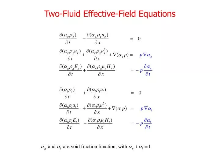
Two-Fluid Effective-Field Equations. Mathematical Issues. Non-conservative: Uniqueness of Discontinuous solution? Pressure oscillations. Non-hyperbolic system: Ill-posedness? Stability Uniqueness. How to sort it out?. Remedy for hyperbolicity: Interfacial pressure correction term and

E N D
Mathematical Issues • Non-conservative: • Uniqueness of Discontinuous solution? • Pressure oscillations • Non-hyperbolic system: Ill-posedness? • Stability • Uniqueness • How to sort it out?
Remedy for hyperbolicity: Interfacial pressure correction term and virtual mass term
Modeling – Interfacial Pressure (IP) Stuhmiller (1977):
Effect of hyperbolicity Solution convergence Faucet Problem: Ransom (1992) • Hyperbolicity insures non-increase of overshoot, but suffering from smearing • Location and strength of void discontinuity is converged, not affected by non-conservative form
Modeling – Virtual Mass (VM) Drew et al (1979)
VM is necessary if IP is not present, the coefficients are unreasonably high for droplet flows. Requirement of VM can be reduced with IP.
Numerical Method • Extended from single-phase AUSM+-up (2003). • Implemented in the All Regime Multiphase Simulator (ARMS). • Cartesian. • Structured adaptive mesh refinement. • Parallelization.
A case with 40% liquid fraction ( Grid size 10cm, calculation time :0-150ms Calculation domain:,L=60m,R=12m ) L=60m Ugas=1km/s R=12m Axis aL=0.4, liquid mass =400kg VL=150m/s(in radial) Liquid area: l=2m, r=0.4m
Liquid fraction, pressure and velocity contours of particle cloud for time 0-150 ms. Lquid fraction (Min:10-8 -Max:10-3) Pressure (Min:1bar-Max:7bar) Gas Velocity (Min:0m/s -Max:1,000m/s)
Current and future works • Complete the hyperbolicity work on the multi-fluid system. • Complete the adaptive mesh refinement into our solver – ARMS • Expand Music-ARMS to solve 3D problems. • Introduce physical models: • Surface tension model • Turbulence model • Verification and validation. • Real world applications.