Query Processing, Resource Management, and Approximation in a Data Stream Management System
Query Processing, Resource Management, and Approximation in a Data Stream Management System. Selected subset of slides taken from talk by Jennifer Widom at NEDS. st anfordst re amdat am anager. Data Streams. Stream = Continuous, unbounded, rapid, time-varying streams of data elements

Query Processing, Resource Management, and Approximation in a Data Stream Management System
E N D
Presentation Transcript
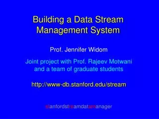
Query Processing, Resource Management, and Approximation in a Data Stream Management System Selected subset of slides taken from talk by Jennifer Widom at NEDS. stanfordstreamdatamanager
Data Streams • Stream = Continuous, unbounded, rapid, time-varying streams of data elements • DSMS = Data Stream Management System
The STREAM System • Declarative language for registering continuous queries; considering data streams and stored relations • Formal semantics; more theoretical team
Contributions to Date • Semantics for continuous queries • Query plans • Exploiting stream constraints • Operator scheduling • Approximation techniques
Streamed Result Stored Result Register Query Input streams Archive The (Simplified) Big Picture DSMS Scratch Store Stored Relations
Archive (Simplified) Network Monitoring Intrusion Warnings Online Performance Metrics Register Monitoring Queries DSMS Network measurements, Packet traces Scratch Store Lookup Tables
Declarative Language for Continuous Queries • A distinction between STREAM and Aurora : • Aurora users directly manipulate one large execution plan • STREAM compiles declarative queries into individual plans, system may merge plans • Syntax based on SQL, additional constructs for sliding windows and sampling
Example Query 1 Two streams, contrived for ease of examples: Orders (orderID, customer, cost) Fulfillments (orderID, clerk)
Example Query 1 Two streams, contrived for ease of examples: Orders (orderID, customer, cost) Fulfillments (orderID, clerk) Total cost of orders fulfilled over the last day by clerk “Sue” for customer “Joe” Select Sum(O.cost) From Orders O, Fulfillments F [Range 1 Day] Where O.orderID = F.orderIDAnd F.clerk = “Sue” And O.customer = “Joe”
Example Query 1 Two streams, contrived for ease of examples: Orders (orderID, customer, cost) Fulfillments (orderID, clerk) Total cost of orders fulfilled over the last day by clerk “Sue” for customer “Joe” Select Sum(O.cost) From Orders O,Fulfillments F [Range 1 Day] Where O.orderID = F.orderIDAnd F.clerk = “Sue” And O.customer = “Joe”
Example Query 1 Two streams, contrived for ease of examples: Orders (orderID, customer, cost) Fulfillments (orderID, clerk) Total cost of orders fulfilled over the last day by clerk “Sue” for customer “Joe” Select Sum(O.cost) From Orders O, Fulfillments F [Range 1 Day] Where O.orderID = F.orderIDAnd F.clerk = “Sue” And O.customer = “Joe”
Example Query 1 Two streams, contrived for ease of examples: Orders (orderID, customer, cost) Fulfillments (orderID, clerk) Total cost of orders fulfilled over the last day by clerk “Sue” for customer “Joe” Select Sum(O.cost) From Orders O, Fulfillments F [Range 1 Day] Where O.orderID = F.orderIDAnd F.clerk = “Sue” And O.customer = “Joe”
Example Query 1 Two streams, contrived for ease of examples: Orders (orderID, customer, cost) Fulfillments (orderID, clerk) Total cost of orders fulfilled over the last day by clerk “Sue” for customer “Joe” Select Sum(O.cost) From Orders O, Fulfillments F [Range 1 Day] Where O.orderID = F.orderIDAnd F.clerk = “Sue” And O.customer = “Joe”
Example Query 2 Using a 10% sample of the Fulfillments stream, take the 5 most recent fulfillments for each clerk and return the maximum cost Select F.clerk, Max(O.cost) From Orders O, Fulfillments F [Partition By clerk Rows 5] 10% Sample Where O.orderID = F.orderID Group By F.clerk
Example Query 2 Using a 10% sample of the Fulfillments stream, take the 5 most recent fulfillments for each clerk and return the maximum cost Select F.clerk, Max(O.cost) From Orders O, Fulfillments F [Partition By clerk Rows 5] 10% Sample Where O.orderID = F.orderID Group By F.clerk
Example Query 2 Using a 10% sample of the Fulfillments stream, take the 5 most recent fulfillments for each clerk and return the maximum cost Select F.clerk, Max(O.cost) From Orders O, Fulfillments F [Partition By clerk Rows 5] 10% Sample Where O.orderID = F.orderID Group By F.clerk
Example Query 2 Using a 10% sample of the Fulfillments stream, take the 5 most recent fulfillments for each clerk and return the maximum cost Select F.clerk, Max(O.cost) From Orders O, Fulfillments F [Partition By clerk Rows 5] 10% Sample Where O.orderID = F.orderID Group By F.clerk
Semantics of Database Languages • An often neglected topic • Traditional relational databases are in reasonable shape • Relational algebra SQL • But triggers were a mess • The semantics of an innocent-looking continuous query over data streams may not be obvious
A Nonobvious Continuous Query • Stream of stock quotes: Stocks(ticker,price) • Monitor last 10 minutes of quotes: Select From Stocks [Range 10 minutes] • Is result a relation, a stream, or something else? • If a relation, what exactly does it contain? • If a stream, how does query differ from: Select From Stocks [Range 1 minute] or Select From Stocks []
Our Semantics and Language for Continuous Queries • Abstract: interpretation for CQs based on certain “black boxes” • Concrete: SQL-based instantiation for our system; includes syntactic shortcuts, defaults, equivalences • Goals • CQs over multiple streams and relations • Exploit relational semantics to the extent possible • Easy queries should be easy to write, simple queries should do what you expect
Relations and Streams • Assume global, discrete, ordered time domain (more on this later) • Relation • Maps time Tto set-of-tuples R • Stream • Set of (tuple,timestamp) elements
Window specification Any relational query language Special operators: Istream, Dstream, Rstream Conversions Streams Relations
Conversion Definitions • Stream-to-relation • S [W] is a relation — at time T itcontains all tuples in window W applied to stream S up to T • When W = , contains all tuples in stream S up to T • Relation-to-stream • Istream(R) contains all (r,T ) where rR at time T but rR at time T–1 • Dstream(R) contains all (r,T ) where rR at time T–1 but rR at time T • Rstream(R) contains all (r,T ) where rR at time T
Abstract Semantics • Take any relational query language • Can reference streams in place of relations • But must convert to relations using any window specification language ( default window = [] ) • Can convert relations to streams • For streamed results • For windows over relations (note: converts back to relation)
Query Result at Time T • Use all relations at time T • Use all streams up to T, converted to relations • Compute relational result • Convert result to streams if desired
Time • Easiest: global system clock • Stream elements and relation updates timestamped on entry to system • Application-defined time • Streams and relation updates contain application timestamps, may be out of order • Application generates “heartbeat” • Or deduce heartbeat from parameters: stream skew, scrambling, latency, and clock progress • Query results in application time
Abstract Semantics – Example 1 Select F.clerk, Max(O.cost) From O [], F [Rows 1000] Where O.orderID = F.orderID Group By F.clerk • Maximum-cost order fulfilled by each clerk in last 1000 fulfillments
Abstract Semantics – Example 1 Select F.clerk, Max(O.cost) From O [], F [Rows 1000] Where O.orderID = F.orderID Group By F.clerk • At time T: entire stream O and last 1000 tuples of F as relations • Evaluate query, update result relation at T
Abstract Semantics – Example 1 Select Istream(F.clerk, Max(O.cost)) From O [], F [Rows 1000] Where O.orderID = F.orderID Group By F.clerk • At time T: entire stream O and last 1000 tuples of F as relations • Evaluate query, update result relation at T • Streamed result: New element (<clerk,max>,T) whenever <clerk,max> changes from T–1
Abstract Semantics – Example 2 Relation CurPrice(stock, price) Select stock, Avg(price) From Istream(CurPrice) [Range 1 Day] Group By stock • Average price over last day for each stock
Abstract Semantics – Example 2 Relation CurPrice(stock, price) Select stock, Avg(price) From Istream(CurPrice) [Range 1 Day] Group By stock • Istream provides history of CurPrice • Window on history, back to relation, group and aggregate
Concrete Language – CQL • Relational query language: SQL • Window spec. language derived from SQL-99 • Tuple-based, time-based, partitioned • Syntactic shortcuts and defaults • So easy queries are easy to write and simple queries do what you expect • Equivalences • Basis for query-rewrite optimizations • Includes all relational equivalences, plus new stream-based ones
Two Extremely Simple CQL Examples Select From Strm • Had better return Strm (It does) • Default window for Strm • Default Istream for result Select From Strm, Rel Where Strm.A = Rel.B • Often want “NOW” window for Strm • But may not want as default
Query Execution • When a continuous query is registered, generation a query plan • Users can also register plans directly • Plans composed of three main components: • Operators (as in most conventional DBMS’s) • Inter-operator Queues (as in many conventional DBMS’s) • State (synopses) • Global scheduler for plan execution
State1 ⋈ State2 Operators and State • State (synopses) • Summarize tuples seen so far (exact or approximate) for operators requiring history • To implement windows • Example: synopsis join • Sliding-window join • Approximation of full join
Simple Query Plan Q1 Q2 State3 ⋈ State4 Scheduler State1 ⋈ State2 Stream3 Stream1 Stream2
Some Issues in Query Plan Generation • Compatibility and conversions for streams and relations (+/- streams) • State sharing, incremental computation • Windowed joins: Multiway versus 2-way • Windows in general: push down, pull up, split, merge, … • Time coordination, operator-level heartbeats
Memory Overhead in Query Processing • Queues + State • Continuous queries keep state indefinitely • Online requirements suggest using memory rather than disk • But we realize this assumption is shaky
Memory Overhead in Query Processing • Queues + State • Continuous queries keep state indefinitely • Online requirements suggest using memory rather than disk • But we realize this assumption is shaky • Goal: minimize memory use while providing timely, accurate answers
Reducing Memory Overhead Two main techniques to date • Exploit constraints on streams to reduce state • Clever operator scheduling to reduce queue sizes
Exploiting Stream Constraints • For most queries, unbounded memory is required for arbitrary streams [PODS ’01]
Exploiting Stream Constraints • For most queries, unbounded memory is required for arbitrary streams [PODS ’01] • But streams may exhibit constraints that reduce, bound, or even eliminate state
Exploiting Stream Constraints • For most queries, unbounded memory is required for arbitrary streams [PODS ’01] • But streams may exhibit constraints that reduce, bound, or even eliminate state • Conventional database constraints • Redefined for streams • “Relaxed” for stream environment
Stream Constraints • Each constraint type defines adherence parameterk • Clustered(k) for attributeS.A • Ordered(k) for attributeS.A • Referential-Integrity(k) for join S1 S2
Algorithm for Exploiting Constraints • Input • Any Select-Project-Join query over streams • Any set of k-constraints • Output • Query execution plan that reduces or eliminates state based on k-constraints • If constraints violated, get approximate result
Constraint Examples Orders (orderID, cost) Fulfillments (orderID, portion, clerk) Query: Many-one join F O
Constraint Examples Orders (orderID, cost) Fulfillments (orderID, portion, clerk) Query: Many-one join F O • Clustered(k) on F.orderID • Matched O tuples discarded after k arrivals of non-matching F’s
Constraint Examples Orders (orderID, cost) Fulfillments (orderID, portion, clerk) Query: Many-one join F O • Clustered(k) on F.orderID • Matched O tuples discarded after k arrivals of non-matching F’s • Referential-Integrity(k) • F tuples retained for at most k arrivals of O tuples
Operator Scheduling • Global scheduler invokes run method of query plan operators with “timeslice” parameter • Many possible scheduling objectives: minimize latency, inaccuracy, memory use, computation, starvation, … • First scheduler: round-robin • Second scheduler: minimize queue sizes • Third scheduler: minimize combination of queue sizes and latency
Approximation • Why approximate? • Memory requirement too high, even with constraints and clever scheduling • Can’t process streams fast enough for query load