Download
1 / 93
930 likes | 956 Views
This resource explores the use of mathematical models for designing and analyzing control systems, focusing on systems like mechanical, hydraulic, and electrical. Topics include linearization, transfer functions, and block diagrams to depict system interconnections. Learn to formulate and solve differential equations for various components and subsystems.

E N D
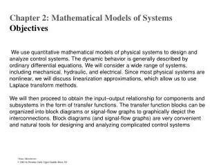
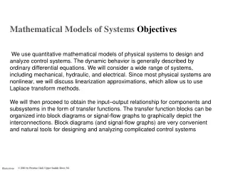
Mathematical Models of Systems Objectives We use quantitative mathematical models of physical systems to design and analyze control systems. The dynamic behavior is generally described by ordinary differential equations. We will consider a wide range of systems, including mechanical, hydraulic, and electrical. Since most physical systems are nonlinear, we will discuss linearization approximations, which allow us to use Laplace transform methods. We will then proceed to obtain the input–output relationship for components and subsystems in the form of transfer functions. The transfer function blocks can be organized into block diagrams or signal-flow graphs to graphically depict the interconnections. Block diagrams (and signal-flow graphs) are very convenient and natural tools for designing and analyzing complicated control systems
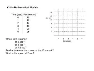
Define the system and its components Formulate the mathematical model and list the necessary assumptions Write the differential equations describing the model Solve the equations for the desired output variables Examine the solutions and the assumptions If necessary, reanalyze or redesign the system Introduction Six Step Approach to Dynamic System Problems
Differential Equation of Physical Systems Energy or Power Electrical Inductance Describing Equation Translational Spring Rotational Spring Fluid Inertia
Differential Equation of Physical Systems Electrical Capacitance Translational Mass Rotational Mass Fluid Capacitance Thermal Capacitance
Differential Equation of Physical Systems Electrical Resistance Translational Damper Rotational Damper Fluid Resistance Thermal Resistance
Linear Approximations • Linear Systems - Necessary condition • Principle of Superposition • Property of Homogeneity • Taylor Series • http://www.maths.abdn.ac.uk/%7Eigc/tch/ma2001/notes/node46.html
The Laplace Transform Historical Perspective - Heaviside’s Operators Origin of Operational Calculus (1887)
Historical Perspective - Heaviside’s Operators Origin of Operational Calculus (1887) v = H(t) Expanded in a power series (*) Oliver Heaviside: Sage in Solitude, Paul J. Nahin, IEEE Press 1987.
The Partial-Fraction Expansion (or Heaviside expansion theorem) Suppose that + The partial fraction expansion indicates that F(s) consists of s z1 F ( s ) a sum of terms, each of which is a factor of the denominator. + × + ( s p1 ) ( s p2 ) The values of K1 and K2 are determined by combining the individual fractions by means of the lowest common denominator and comparing the resultant numerator or coefficients with those of the coefficients of the numerator before separation in different terms. K1 K2 + F ( s ) + + s p1 s p2 Evaluation of Ki in the manner just described requires the simultaneous solution of n equations. An alternative method is to multiply both sides of the equation by (s + pi) then setting s= - pi, the right-hand side is zero except for Ki so that + × + ( s pi ) ( s z1 ) s = - pi Ki + + + ( s p1 ) ( s p2 ) The Laplace Transform
The Laplace Transform Useful Transform Pairs
The Laplace Transform Consider the mass-spring-damper system
The Transfer Function of Linear Systems Example 2.2
Block Diagram Models Original Diagram Equivalent Diagram Original Diagram Equivalent Diagram
Block Diagram Models Original Diagram Equivalent Diagram Original Diagram Equivalent Diagram
Block Diagram Models Original Diagram Equivalent Diagram Original Diagram Equivalent Diagram