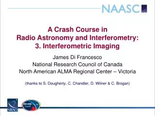
A Crash Course in Radio Astronomy and Interferometry : 3. Interferometric Imaging

A Crash Course inRadio Astronomy and Interferometry:3. Interferometric Imaging James Di Francesco National Research Council of Canada North American ALMA Regional Center – Victoria (thanks to S. Dougherty, C. Chandler, D. Wilner & C. Brogan)

Aperture Synthesis Aperture Synthesis • sample V(u,v) at enough points to synthesize the equivalent large aperture of size (umax,vmax) • 1 pair of telescopes  1 (u,v) sample at a time • N telescopes number of samples = N(N-1)/2 • fill in (u,v) plane by making use of Earth rotation: Sir Martin Ryle, 1974 Nobel Prize in Physics • reconfigure physical layout of N telescopes for more Sir Martin Ryle 1918-1984 2 configurations of 8 SMA antennas 345 GHz Dec = -24 deg

Imaging (u,v) Plane Sampling • in aperture synthesis, V(u,v) samples are limited by number of telescopes, and Earth-sky geometry • high spatial frequencies: • maximum angular resolution • low spatial frequencies: • extended structures invisible • (aka. only a max scale can be imaged; also ``zero-spacing problem” = no large scales) • irregular within high/low limits: • sampling theorem violated • still more information missing

Imaging Formal Description dij(u,v) • sample Fourier domain at discrete points, i.e., • so, the inverse Fourier transform of the ensemble of visibilities is: • but the convolution theorem tells us: where (the point spread function) Fourier transform of sampled visibilities yields the true sky brightness convolved with the point spread function (the “dirty image” is the true image convolved with the “dirty beam”) I I I

Imaging Dirty Beam and Dirty Image b(x,y) (dirty beam) B(u,v) ID(x,y) (dirty image) I(x,y)

Imaging Dirty Beam Shape and N Antennas 2 Antennas

Imaging Dirty Beam Shape and N Antennas 8 Antennas x 6 Samples

Imaging How to analyze interferometer data? • uv plane analysis • best for “simple” sources, e.g., point sources, disks • image plane analysis • Fourier transform V(u,v) samples to image plane, getID(x,y) • but difficult to do science on dirty image • deconvolveb(x,y) fromID(x,y) to determine (model of)I(x,y) visibilities dirty image sky brightness deconvolve Fourier transform

Imaging Weighting and Tapering • Visibility Weighting in the FT: • Including weighting function W to modify dirty beam sidelobes: • natural weighting: density of uv-coverage = highest compact flux sensitivity • uniform weighting: extent of uv-coverage = highest resolution • robust weighting: compromise between natural and uniform • tapering: downweights high spatial frequencies = higher extended flux sensitivity • imaging parameters provide a lot of freedom • appropriate choice depends on science goals • recall that the primary beam FWHM is the “field-of-view” of a single-pointing interferometric image

Imaging Weighting and Tapering: Examples Robust 0 0.41x0.36 = 1.6 Natural 0.77x0.62 = 1.0 Robust 0 + Taper 0.77x0.62 = 1.7 Uniform 0.39x0.31 = 3.7

Field of View: Single Pointing FOV [12 m] Band 3 (54”) ~4’ Band 6 (27”) Band 7 (18”) Band 9 (9”) B68 ALMA single pointing

Field of View: Mosaics Nyquist Spacing = 3-1/2 (/D) rad. = 29.75” x (/100 GHz)-1 =constant rms over inner area Mosaics of up to 50 pointings OK for Early Science ~4’ B68 ALMA Band 3 mosaic

Next: Deconvolution

A Crash Course in Radio Astronomy and Interferometry : 3. Interferometric Imaging