Download
1 / 13
130 likes | 308 Views
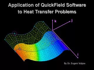
Application of QuickField Software to Heat Transfer Problems. j. k. i. By Dr. Evgeni Volpov. Basic Formulations for GIS HT model. Classical Heat Transfer Equations. Boundary Conditions. 1. T(S) = T 0 Const Temperature T(S) = T 0 + k.S Linear Temp.

E N D
Application of QuickField Softwareto Heat Transfer Problems j k i By Dr. Evgeni Volpov
Basic Formulations for GIS HT model Classical Heat Transfer Equations Boundary Conditions 1. T(S) = T0 Const Temperature T(S) = T0 + k.S Linear Temp. 2. Fn = -qs Flux Fn(+) - Fn(-) = -qs 3. Fn = a(T - T0) Convection a - film coefficient T0– temperature of contacting medium 4. Fn = b.Ksb(T4 - T04) Radiation Ksb - Stephan-Boltzmann constant; b - emissivity coefficient
Boundary conditions & domain characterization Surface element Volume element Point-Source element
Coupling Problems solution for SF6 GIS 170 kV enclosure 1920 W/m3 epoxy spacer 500 W/m3 2.3 MV/m Joule losses distribution at central conductor 1000 A 100 kV AC Electric Field distribution in GIS compartment 31 C enclosure P SF6 = 0.6 MPa epoxy spacer Air Spacer deformation under SF6 pressure 53 C HV conductor current 1000 A Thermo-static field mapping in GIS compartment
SF6 GIS HT Model Parameters 1. SF6 Thermal Conductivityg = 0.0136 W/m.K 2. Air Thermal Conductivitya = 0.026 W/m.K 3. Epoxy Thermal Conductivitye (0.3-0.6) W/m.K 4. Aluminum Thermal Conductivityal (140-220) W/m.K 5. Copper Thermal Conductivitycu = 380 W/m.K 6. Convection Parameters: 6.1. Internal SF6 space: k= 0.133(Gr.Pr)0.28 (1.2 - 6.0) 103 < Gr.Pr < 106(for SF6 GIS) 6.2. External Air space: ac (2-10) W/K.m2 ; T0 (20-25C) 7. Radiation Parameters: equivalent emissivity coefficient: be (0.01 - 0.6)
GIS Geometric Model examples Symmetry Axis (a) L Hot-spot Air layer L (b)
Geometric Models & results presentation r - Z - r
Thermal Field mapping for BB model 1.2 m T0 (ambient) = 20C Conductivity only 23.8 C 23.0 C 1000 A 64 C 63.0 C Hot-spot Flange Conductivity + convection 29.8C 28.8C 1000 A 64 C 60.1 C Conductivity + convection+ radiation 29.7 C 28.1 C 1000 A 64 C 54.0 C 1.2 m
Thermal Field mapping for BB model 2.3 m T0 (ambient) = 20C Conductivity only 23.9 C 23.1 C 1000 A 64 C 62.6 C Hot-spot Conductivity + convection 31.0 C 29.1 C 1000 A 64 C 54.1 C Flange Conductivity + convection+ radiation 29.5 C 26.8 C 1000 A 64 C 43.0 C 2.3 m
Enclosure overheating as a function of Hot-spot temperature T C Temperature drop along the enclosure BB length 1 m Hot-spot temperature Tmax C BB length 2 m Including radiation
Enclosure overheating as a function of the BB length R = 100 I = 1000 A V = 1000 cm3 Specific Joule loss in the damaged contact Tmax C 100 kW/m3 50 kW/m3 Max temperature on the enclosure Enclosure temperature with no damaged contact Enclosure length L [m] T0 (ambient) = 20C Conductivity + convection Conductivity + convection+ radiation
HT Transients for BB model T C T0 (ambient) = 20C 2.3 m 0 A Initial distribution 3 2.6 10 5 sec Q2 = 2 kW/m3 Q1 = 100 kW/m3 1000 A Steady State distribution T C Conductivity + convection g k = 0.10