Download
1 / 41
420 likes | 685 Views
Fig. 14.1. 14. Stochastic Processes. Introduction. Let denote the random outcome of an experiment. To every such outcome suppose a waveform is assigned. The collection of such waveforms form a stochastic process. The set of and the time

E N D
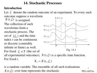
Fig. 14.1 14. Stochastic Processes Introduction Let denote the random outcome of an experiment. To every such outcome suppose a waveform is assigned. The collection of such waveforms form a stochastic process. The set of and the time index t can be continuous or discrete (countably infinite or finite) as well. For fixed (the set of all experimental outcomes), is a specific time function. For fixed t, is a random variable. The ensemble of all such realizations over time represents the stochastic PILLAI/Cha
process X(t). (see Fig 14.1). For example where is a uniformly distributed random variable in represents a stochastic process. Stochastic processes are everywhere: Brownian motion, stock market fluctuations, various queuing systems all represent stochastic phenomena. If X(t) is a stochastic process, then for fixed t, X(t) represents a random variable. Its distribution function is given by Notice that depends on t, since for a different t, we obtain a different random variable. Further represents the first-order probability density function of the process X(t). (14-1) (14-2) PILLAI/Cha
For t = t1 and t = t2, X(t) represents two different random variables X1 = X(t1) and X2 = X(t2) respectively. Their joint distribution is given by and represents the second-order density function of the process X(t). Similarly represents the nth order density function of the process X(t). Complete specification of the stochastic process X(t) requires the knowledge of for all and for all n. (an almost impossible task in reality). (14-3) (14-4) PILLAI/Cha
Mean of a Stochastic Process: • represents the mean value of a process X(t). In general, the mean of • a process can depend on the time index t. • Autocorrelation function of a process X(t) is defined as • and it represents the interrelationship between the random variables • X1 = X(t1) and X2 = X(t2) generated from the process X(t). • Properties: • 2. (14-5) (14-6) (14-7) (Average instantaneous power) PILLAI/Cha
3. represents a nonnegative definite function, i.e., for any set of constants Eq. (14-8) follows by noticing that The function represents the autocovariance function of the process X(t). Example 14.1 Let Then (14-8) (14-9) (14-10) PILLAI/Cha
Example 14.2 (14-11) This gives (14-12) Similarly (14-13) PILLAI/Cha
Stationary Stochastic Processes Stationary processes exhibit statistical properties that are invariant to shift in the time index. Thus, for example, second-order stationarity implies that the statistical properties of the pairs {X(t1) , X(t2) } and {X(t1+c) , X(t2+c)} are the same for anyc. Similarly first-order stationarity implies that the statistical properties of X(ti) and X(ti+c) are the same for any c. In strict terms, the statistical properties are governed by the joint probability density function. Hence a process is nth-order Strict-Sense Stationary (S.S.S) if for anyc, where the left side represents the joint density function of the random variables and the right side corresponds to the joint density function of the random variables A process X(t) is said to be strict-sense stationary if (14-14) is true for all (14-14) PILLAI/Cha
For a first-order strict sense stationary process, from (14-14) we have for any c. In particular c = – t gives i.e., the first-order density of X(t) is independent of t. In that case Similarly, for a second-order strict-sense stationary process we have from (14-14) for any c. For c = – t2 we get (14-15) (14-16) (14-17) (14-18) PILLAI/Cha
i.e., the second order density function of a strict sense stationary process depends only on the difference of the time indices In that case the autocorrelation function is given by i.e., the autocorrelation function of a second order strict-sense stationary process depends only on the difference of the time indices Notice that (14-17) and (14-19) are consequences of the stochastic process being first and second-order strict sense stationary. On the other hand, the basic conditions for the first and second order stationarity – Eqs. (14-16) and (14-18) – are usually difficult to verify. In that case, we often resort to a looser definition of stationarity, known as Wide-Sense Stationarity (W.S.S), by making use of (14-19) PILLAI/Cha
(14-17) and (14-19) as the necessary conditions. Thus, a process X(t) • is said to be Wide-Sense Stationary if • and • (ii) • i.e., for wide-sense stationary processes, the mean is a constant and • the autocorrelation function depends only on the difference between • the time indices. Notice that (14-20)-(14-21) does not say anything • about the nature of the probability density functions, and instead deal • with the average behavior of the process. Since (14-20)-(14-21) • follow from (14-16) and (14-18), strict-sense stationarity always • implies wide-sense stationarity. However, the converse is not true in • general, the only exception being the Gaussian process. (14-20) (14-21) PILLAI/Cha
for wide sense stationarity, we obtain strict sense stationarity as well. From (14-12)-(14-13), (refer to Example 14.2), the process in (14-11) is wide-sense stationary, but not strict-sense stationary. Similarly if X(t) is a zero mean wide sense stationary process in Example 14.1, then in (14-10) reduces to As t1, t2 varies from –T to +T, varies from –2T to + 2T. Moreover is a constant over the shaded region in Fig 14.2, whose area is given by and hence the above integral reduces to Fig. 14.2 (14-24) PILLAI/Cha
Systems with Stochastic Inputs A deterministic system1 transforms each input waveform into an output waveform by operating only on the time variable t. Thus a set of realizations at the input corresponding to a process X(t) generates a new set of realizations at the output associated with a new process Y(t). Fig. 14.3 Our goal is to study the output process statistics in terms of the input process statistics and the system function. 1A stochastic system on the other hand operates on both the variables t and PILLAI/Cha
Deterministic Systems Memoryless Systems Systems with Memory Time-Invariant systems Linear systems Time-varying systems Fig. 14.3 Linear-Time Invariant (LTI) systems LTI system PILLAI/Cha
Memoryless Systems: The output Y(t) in this case depends only on the present value of the input X(t). i.e., (14-25) Strict-sense stationary input Memoryless system Strict-sense stationary output. (see (9-76), Text for a proof.) Need not be stationary in any sense. Wide-sense stationary input Memoryless system Y(t) stationary,but not Gaussian with (see (14-26)). X(t) stationary Gaussian with Memoryless system Fig. 14.4 PILLAI/Cha
Linear Systems: represents a linear system if Let represent the output of a linear system. Time-Invariant System: represents a time-invariant system if i.e., shift in the input results in the same shift in the output also. If satisfies both (14-28) and (14-30), then it corresponds to a linear time-invariant (LTI) system. LTI systems can be uniquely represented in terms of their output to a delta function (14-28) (14-29) (14-30) Impulse response of the system LTI Fig. 14.5 Impulse response Impulse PILLAI/Cha
then LTI Fig. 14.6 arbitrary input (14-31) Eq. (14-31) follows by expressing X(t) as and applying (14-28) and (14-30) to Thus (14-32) By Linearity By Time-invariance (14-33) PILLAI/Cha
Output Statistics:Using (14-33), the mean of the output process is given by Similarly the cross-correlation function between the input and output processes is given by Finally the output autocorrelation function is given by (14-34) (14-35) PILLAI/Cha
(14-36) or (14-37) h(t) (a) h*(t2) h(t1) (b) Fig. 14.7 PILLAI/Cha
In particular if X(t) is wide-sense stationary, then we have so that from (14-34) Also so that (14-35) reduces to Thus X(t) and Y(t) are jointly w.s.s. Further, from (14-36), the output autocorrelation simplifies to From (14-37), we obtain (14-38) (14-39) (14-40) (14-41) PILLAI/Cha
From (14-38)-(14-40), the output process is also wide-sense stationary. This gives rise to the following representation wide-sense stationary process LTI system h(t) wide-sense stationary process. (a) strict-sense stationary process LTI system h(t) strict-sense stationary process (see Text for proof ) (b) Linear system Gaussian process (also stationary) Gaussian process (also stationary) (c) Fig. 14.8 PILLAI/Cha
White Noise Process: W(t) is said to be a white noise process if i.e., E[W(t1) W*(t2)] = 0 unless t1 = t2. W(t) is said to be wide-sense stationary (w.s.s) white noise if E[W(t)] = constant, and If W(t) is also a Gaussian process (white Gaussian process), then all of its samples are independent random variables (why?). For w.s.s. white noise input W(t), we have (14-42) (14-43) LTI h(t) White noise W(t) Fig. 14.9 PILLAI/Cha
and where Thus the output of a white noise process through an LTI system represents a (colored) noise process. Note: White noise need not be Gaussian. “White” and “Gaussian” are two different concepts! (14-44) (14-45) (14-46) PILLAI/Cha
Discrete Time Stochastic Processes: A discrete time stochastic process Xn = X(nT) is a sequence of random variables. The mean, autocorrelation and auto-covariance functions of a discrete-time process are gives by and respectively. As before strict sense stationarity and wide-sense stationarity definitions apply here also. For example, X(nT) is wide sense stationary if and (14-57) (14-58) (14-59) (14-60) (14-61) PILLAI/Cha
From (14-64), if X(nT) is a wide sense stationary stochastic process then Tn is a non-negative definite matrix for every Similarly the converse also follows from (14-64). (see section 9.4, Text) If X(nT) represents a wide-sense stationary input to a discrete-time system {h(nT)}, and Y(nT) the system output, then as before the cross correlation function satisfies and the output autocorrelation function is given by or Thus wide-sense stationarity from input to output is preserved for discrete-time systems also. (14-64) (14-65) (14-66) (14-67) PILLAI/Cha
18. Power Spectrum For a deterministic signal x(t), the spectrum is well defined: If represents its Fourier transform, i.e., if then represents its energy spectrum. This follows from Parseval’s theorem since the signal energy is given by Thus represents the signal energy in the band (see Fig 18.1). (18-1) (18-2) Energy in Fig 18.1 PILLAI
However for stochastic processes, a direct application of (18-1) generates a sequence of random variables for every Moreover, for a stochastic process, E{| X(t) |2} represents the ensemble average power (instantaneous energy) at the instant t. PILLAI
to be the power spectral density of the w.s.s process X(t). Notice that i.e., the autocorrelation function and the power spectrum of a w.s.s Process form a Fourier transform pair, a relation known as the Wiener-Khinchin Theorem. From (18-8), the inverse formula gives and in particular for we get From (18-10), the area under represents the total power of the process X(t), and hence truly represents the power spectrum. (Fig 18.2). (18-7) (18-8) (18-9) (18-10) PILLAI
If X(t) is a real w.s.s process, then so that so that the power spectrum is an even function, (in addition to being real and nonnegative). (18-13) PILLAI
Power Spectra and Linear Systems If a w.s.s process X(t) with autocorrelation function is applied to a linear system with impulse response h(t), then the cross correlation function and the output autocorrelation function are given by (14-40)-(14-41). From there But if Then since h(t) X(t) Y(t) Fig 18.3 (18-14) (18-15) (18-16) PILLAI
Using (18-15)-(18-17) in (18-14) we get since where represents the transfer function of the system, and (18-17) (18-18) (18-19) (18-20) PILLAI
From (18-18), the cross spectrum need not be real or nonnegative; However the output power spectrum is real and nonnegative and is related to the input spectrum and the system transfer function as in (18-20). Eq. (18-20) can be used for system identification as well. W.S.S White Noise Process: If W(t) is a w.s.s white noise process, then from (14-43) Thus the spectrum of a white noise process is flat, thus justifying its name. Notice that a white noise process is unrealizable since its total power is indeterminate. From (18-20), if the input to an unknown system in Fig 18.3 is a white noise process, then the output spectrum is given by Notice that the output spectrum captures the system transfer function characteristics entirely, and for rational systems Eq (18-22) may be used to determine the pole/zero locations of the underlying system. (18-21) (18-22) PILLAI
Example 18.1: A w.s.s white noise process W(t) is passed through a low pass filter (LPF) with bandwidth B/2. Find the autocorrelation function of the output process. Solution: Let X(t) represent the output of the LPF. Then from (18-22) Inverse transform of gives the output autocorrelation function to be (18-23) (18-24) (a) LPF (b) Fig. 18.4 PILLAI
Eq (18-23) represents colored noise spectrum and (18-24) its autocorrelation function (see Fig 18.4). Example 18.2: Let represent a “smoothing” operation using a moving window on the input process X(t). Find the spectrum of the output Y(t) in term of that of X(t). Solution: If we define an LTI system with impulse response h(t) as in Fig 18.5, then in term of h(t), Eq (18-25) reduces to so that Here (18-25) Fig 18.5 (18-26) (18-27) (18-28) PILLAI
so that (18-29) Fig 18.6 Notice that the effect of the smoothing operation in (18-25) is to suppress the high frequency components in the input and the equivalent linear system acts as a low-pass filter (continuous- time moving average) with bandwidth in this case. PILLAI
turns out to be the overall matched filter for the original problem. Once again, transmit signal design can be carried out in this case also. AM/FM Noise Analysis: Consider the noisy AM signal and the noisy FM signal where (18-65) (18-66) (18-67) (18-68) PILLAI
Here m(t) represents the message signal and a random phase jitter in the received signal. In the case of FM, so that the instantaneous frequency is proportional to the message signal. We will assume that both the message process m(t) and the noise process n(t) are w.s.s with power spectra and respectively. We wish to determine whether the AM and FM signals are w.s.s, and if so their respective power spectral densities. Solution:AM signal: In this case from (18-66), if we assume then so that (see Fig 18.15) (18-69) (18-70) (a) (b) Fig 18.15 PILLAI
Thus AM represents a stationary process under the above conditions. What about FM? FM signal: In this case (suppressing the additive noise component in (18-67)) we obtain since (18-71) PILLAI
Eq (18-71) can be rewritten as where and In general and depend on both t and so that noisy FM is not w.s.s in general, even if the message process m(t) is w.s.s. In the special case when m(t) is a stationary Gaussian process, from (18-68), is also a stationary Gaussian process with autocorrelation function for the FM case. In that case the random variable (18-72) (18-73) (18-74) (18-75) PILLAI
where Hence its characteristic function is given by which for gives where we have made use of (18-76) and (18-73)-(18-74). On comparing (18-79) with (18-78) we get and so that the FM autocorrelation function in (18-72) simplifies into (18-76) (18-77) (18-78) (18-79) (18-80) (18-81) PILLAI
Notice that for stationary Gaussian message input m(t) (or ), the nonlinear output X(t) is indeed strict sense stationary with autocorrelation function as in (18-82). Narrowband FM: If then (18-82) may be approximated as which is similar to the AM case in (18-69). Hence narrowband FM and ordinary AM have equivalent performance in terms of noise suppression. Wideband FM: This case corresponds to In that case a Taylor series expansion or gives (18-82) (18-83) PILLAI
and substituting this into(18-82) we get so that the power spectrum of FM in this case is given by where Notice that always occupies infinite bandwidth irrespective of the actual message bandwidth (Fig 18.16)and this capacity to spread the message signal across the entire spectral band helps to reduce the noise effect in any band. (18-84) (18-85) (18-86) (18-87) Fig 18.16 PILLAI