Download
1 / 30
300 likes | 332 Views
This study examines the features of turbulence during the polar winter at Dome C, Antarctica. The correlation between turbulence behavior and meteorological conditions is determined, and wavelike structures are analyzed. The results provide insight into extreme stable stratification and the characteristics of turbulence in this environment.

E N D
Spatio-temporal Pattern of the Surface-based Turbulent Layer during Polar Winter at Dome C, Antarctica as observed by Sodar I. Petenko1,2,S. Argentini1, G. Mastrantonio1,A. Viola1, M. Kallistratova2, G. Casasanta1, A. Conidi1, R. Sozzi3 1Institute ofAtmosphericSciences and Climate, CNR, Via Fosso del Cavaliere 100, 00133, Roma, Italy.E-mail: i.petenko@isac.cnr.it 2A.M.Obukhov Institute of Atmospheric Physics, RAS, Pyzhevskiy 3, 109117, Moscow, Russia 3Regional Environmental Protection Agency of Lazio, Via Boncompagni 101, 00187 – Roma, Italy
OUTLINE of the Presentation • 1. Scientific motivations and objectives • 2. Site and instrumentation • 3. Occurrence and features of turbulent layers • 4. Correlation between the depth of turbulent layers and meteorological parameters • 5. Wavelike structures and their characteristics • 6. Summary
Scientific Objectives • 1.Study the features of turbulence under extremelystable stratification observedduring polar winter • 2. Determine the correlation between the turbulencebehaviour and meteorological conditions • 3. Determine the wavelike structure • features
Experimental Site French-Italian station of Concordia Dome C, Antarctica 75°S, 123°E, 3233 m a.s.l. We will see the features of atmospheric turbulence during the austral winter of 2012 in the interior of Antarctica
Experimental Set-up SODAR surface-layerhigh-resolution sodar measures a spatio-temporalstructure of thermalturbulencebeginning from ≈2 m up to 200 m with a verticalresolution<2 m, and a time resolution of 2 s. 1) Ultrasonic anemometer USA-1 by Metek 2) Net Radiometer CNR1 by Kipp & Zonen AWS Milos520 by Vaisaala Radiosonde RS92-SGPL The experiment was held from December 2011 to December 2012 Frequency: 4850 Hz Pulse duration : 0.01 s Pulse repetition: 2 s Description of the sodar and preliminaryresults: Argentini S., I. Petenko, et al. (2014) The surface layer observed by a high resolution sodar at Dome C, Antarctica. Annals of Geophysics, 56, 5; 10.4401/ag-6347.
Features of the Presented Results “Quasi-LABORATORY” experiment – minimally influenced by external factors 1. Horizontal HOMOGENEITY - NO OROGRAPHY influence (flat surface with a slope < 0.1%) 2. NO external HEAT sources (almost no Sun) 3. (almost) NO DIURNAL VARIATIONS 4. Long-term measurements during several months – statistics is reliable
What does SODAR show? Sodar echograms show cross-section of the spatial and temporal pattern of thermal turbulence in height-time coordinates. The greyscale intensity (or conditional colours) is proportional to the Temperature Structure Parameter CT2 Surface-basedTurbulentLayer (STL) asshown by sodar The DEPTH of the STL is a HEIGHT of the top boundary
Variation of the STL Depth in Winter of 2012 Occurrence of Surface Turbulent Layer Depth: 0-10 m 33% 10-30 m 37% 30-50 m 17% > 50 m 13%
Depths of the Surface-based Turbulent Layer (from sodar) and of the Inversion Layer (from radiosonde) Surface-based Turbulent Layer occupies only the lowest 10-20% of a whole temperature inversion layer. This is the main difference between the turbulence in the long-lived stable boundary layer and the usual nocturnal inversion layer
Meteorological Conditions for different STL Depths “Shallow” STL, Depth 0-10 m, 836 hours – 33% “Deep” STL, Depth 30-50 m, 438 hours – 17%
STL Depth vs Wind Speed and Temperature Height 1.4 m Height 3.5 m The depth of the Surface-based Turbulent Layer increases with Wind Speed, and shows weak dependence on temperature
Variation of STL vs Meteorological Parameters Shallow STL and Weak Turbulence Temperature Wind Speed & Direction Deep STL and Strong Turbulence Temperature Wind Speed & Direction
Wavelike Patterns in Antarctica Wavelike patterns are often observed in the interrior of Antarctica, from the surface to the upper atmospheric layers
Example of long-lived STL with WAVY internal structure (WAVE TRAINS) V= 7 m/s S, T= -65°C Wavy braid parttern can be associated with gravity-shear waves due to the Kelvin-Helmholtz instability
Example of long-lived STL with UNIFORM internal structure V= 5 m/s S, T= -65°C
Spectral Characteristics of Wave Trains Low-Frequency part P1 is the period of trains High-Frequency part P2 is the period of waves P2 ≈ 20 s P1≈ 700 s For the temperature gradient of 6.5°C/km measured by the radiosonde in the free atmosphere, buoyancy period ≈ 520 s
Classification of STL STL can be characterized by its DEPTH and INTERNAL STRUCTURE The observed STLs can be subdivided into several groups according to their depth and internal structure. “Shallow”: 1) Depth <20 m without any visible regularity of the internal structure. 2) Depth <20 m with a wavy internal sub-layer. “Deep”: 1) Depth of 20-60 m with uniform internal structure 2) Depth of 20-60 m with wavy internal structure of a braid form with periods of 60-300 s (Kelvin-Helmoholtz instability) 3) Depth of >60 m with wavy internal structure with periods of 60-120 s through the whole depth 4)*Depth of 30-60 m with periodical (of ≈10-12 minutes) alternation of wave trains (with internal periods of ≈20-30 s and duration of ≈4-5 minutes) and zones with uniform internal structure. * This case is more complicate and often occurs.
Features of Turbulence in Winter at Dome C: • In spite of • the absence of the Sun and very low temperatures, • extremely high static stability and strong temperature inversion extending up to 100-300 m with a strength reaching 30-40°C, • the absence of orographyfeatures • relatively long periods of steady weather conditions • TURBULENCE is quite VIVID and LIVELY • and shows • different and variable spatio-temporal structures
Applicationfor Astronomy Correlation between Seeing and STL Depth The intensity of thermal turbulence measured by a sodar is characterized by the temperature structure parameter CT2. The intensity of optically-active turbulence is described by the refraction index structure parameterCn2. These parameters are connected directly Cn2(h)= B(p, T) CT2(h) The coefficient B(p, T)= (79.2∙10-6pT-2)2 , where p is the air pressure in mb, T is the absolute temperature in K. The Turbulent Optical Factor (TOF) TOF = ∫Cn2(h)dh evaluates a degree of degradation of a stellar image by turbulence localized in the layer at altitudes from h1 to h2. The best image quality (lowest seeing) is observed for lower STL depth Correlation between Seeing and TOF The best image quality (lowest seeing) is observed for lower TOF values Petenko, I. et al. (2014) Observations of optically active turbulence in the planetary boundary layer by sodar at the Concordia astronomical observatory, Dome C, Antarctica. Astronomy & Astrophys, A 568, A44 (2014)
SUMMARY Considerable thermal turbulence often occurs and extends up to several tens of metres forming the Surface-based Turbulent Layer (STL) at the Antarctic plateau during the austral winter. The STL occupies only the lowest 10-20% of the whole temperature-inversion layer. The STL depth increases with wind speed. Wind Speed seems to be the most relevant variable influencing the structure and intensity of thermal turbulence in the polar STL. Distinct wave activity within the STL occurs during a large part of the time and can be assumed to be the main feature of the STL occurring under very stable stratification. Classification of typical patterns of the spatio-temporal structure of turbulence observed by the use of the advanced high-resolution sodar is presented
Thank you • Благодаря • Merci • Danke • Gracias • Grazie • Спасибо
Example of long-lived STL with WAVY internal structure V= 9 m/s S, T= -60°C
Example of long-lived STL with WAVY internal structure (WAVE TRAINS) V= 6 m/s S, T= -65°C
Example of long-lived STL with WAVY internal structure (WAVE TRAINS) V= 6 m/s S, T= -65°C
Cross-section patterns of the Surface–based Turbulent Layer (STL) shown by sodar echograms Greyscale intensity is proportional to the strength of thermal turbulence characterised by the temperature structure parameter CT2 Typical profiles of CT2 within STL
Variation of STL vs Meteorological Parameters Low STL and Weak Turbulence
Variation of STL vs Meteorological Parameters High STL and Strong Turbulence
Variation of STL vs Meteorological Parameters Variable STL and Strong Turbulence