Download

1 / 45
450 likes | 473 Views
Review and Rating Discharge Measurements. David S. Mueller Office of Surface Water March 2010. Overview. Considerations in Rating a Measurement Six Review Steps Gather information for rating as you review Three Examples. Rating Process.

E N D
Review and Rating Discharge Measurements David S. Mueller Office of Surface Water March 2010
Overview • Considerations in Rating a Measurement • Six Review Steps • Gather information for rating as you review • Three Examples
Rating Process • Quantitative assessment of measurement uncertainty • Currently being worked on • Current practice is subjective • Where we can quantify we will • Where we can’t we will make qualitative estimates
Rating Considerations • Variability of transect discharges • Pattern in transect discharges • Accuracy of top and bottom extrapolation • Accuracy of edge extrapolation • Quantity and distribution of missing data • Quality of boat navigation reference • Bias or noise in bottom track • Noise in GPS data
Spread in Transect Discharges • A coefficient of variation (COV) is computed by the software (Std./|Avg.|) • The COV represents the sampled random error in the discharge measurement. • Dividing the COV by the sqrt of the number of passes and multiplying by the correct value will provide the 95% uncertainty associated with random errors as measured • For 4 passes: 1.6*COV • For 8 passes: 0.8*COV • This does not include any bias errors • This is probably and optimistic estimate
Example of Random Error 95% Uncertainy (Random Error) = 0.05*0.8 = 4%
Patterns in Transects • Random errors should not display a pattern • A pattern in flow may indicate the need to adjust measurement procedures • Rapidly rising or falling – average fewer transects • Periodic – use more transects to capture variability
Top Extrapolation • Average appropriate number of ensembles • Evaluate discharge profile • Check field notes for wind effects • Try different extrapolation methods and compare change in total discharge • Little change – accurate extrapolation likely • Significant change – how good is the data on which the selection is made • Surface effects captured? • Field notes consistent with pattern? • What percentage of flow is in the top portion • Subjective judgment
Bottom Extrapolation • Smooth streambed • Accurate extrapolation likely • Rough streambed • Extrapolation uncertain
Edge Estimates • What percentage of flow is in the edges? • May be small enough to disregard accuracy • Recommend no more than 5% in each edge • Subjective judgment • Large edge estimates • Irregular edge shapes Edge Q = 25% of total
Invalid Data • Percent of invalid data • Distribution of invalid data • How well is that portion of the flow estimated
Summary of Rating Approach • Consider the data • Consider the hydraulics • Consider site conditions • Use statistics, if possible • Use your judgment • Pay attention to potential errors (as a percentage) as you review the data
Steps of Review • QA/QC • Composite tabular • Stick Ship Track • Velocity contour • Extrapolation • Discharge summary
QA/QC • ADCP Test Error Free? • Compass Calibration • Calibration and evaluation completed • < 1 degree error • Important for Loop and GPS • Moving-Bed Test • Loop • Requires compass calibration • Use LC to evaluate • Stationary • Duration and Deployment • SMBA required to evaluate StreamPro
Composite Tabular • Number of Ensembles • > 150 ??? • Lost Ensembles • Communications error • Bad Ensembles • Distribution more important than percentage • Distribution evaluated in velocity contour plot • Reasonable temperature
Stick Ship Track • Check with appropriate reference (BT, GGA, VTG) • Track and sticks in correct direction • Magnetic variation • Heading time series • Sticks representative of flow • WT thresholds • Irregular ship track? • BT thresholds • BT 4-beam solutions
Velocity Contour • Patterns in velocity distribution • Nonuniform • Unnatural • WT Thresholds • Spikes in bottom profile • Turn on Screen Depth • Distribution of invalid and unmeasured areas • Qualitative assessment of uncertainty
Velocity Extrapolation • Average ensembles (10-20) • Evaluate several transects • Use Power/Power as default • Find reasons to deviate from Power/Power • Don’t waste time where there is little difference • In doubt try different options an evaluate change in discharge • Helps evaluate potential uncertainty from extrapolation • Person collecting data gets benefit of doubt
Discharge Summary • Transects within 5% • Directional bias • GPS used • Magvar correction • Consistency • Discharges (top, meas., bottom, left, right) • Width, Area • Boat speed, Flow Speed, Flow Dir.
Example 1 – Compass Cal. • Compass Evaluation is Good!
Example 1 – Moving-Bed Test • Loop looks good • LC finds no problems with loop • Lost BT • Compass Error • No moving-bed correction required
Example 1 – Composite Tabular • > 300 ensembles • No lost ensembles • 0-1 bad ensembles • Temperature reasonable
Example 1 – Ship Track / Contour • Ship track consistent • No spikes in streambed in contour plot • No hydraulically unusual patterns • Unmeasured areas reasonable in size
Example 1 - Extrapolation • Top extrapolation a bit uncertain • Try Power/Power • Changed Q = 0.6% • Const / No Slip = OK
Example 1 – Discharge Summary • All within 5% • 1 negative Q in left edge • Everything else very consistent
Example 1 - Rating • Base uncertainty • 1.6*0.01= 1.6% • Invalid Data • None • Extrapolation • 0.5-1% uncertainty in extrapolation • Top is only about 10% of total • Edges • About 1% of total Q • Final assessment • Rate this measurement “GOOD”
Example 2 – QA/QC • No test errors • Compass Cal • High pitch and roll • Moving-bed tests • Bottom track problems
Example 2 – Bottom Track Issue • Time series plots show spikes • 3-beam solution • High vertical velocity
Example 2 – Composite Tabular • Too few ensembles • Short duration • Bad ensembles
Example 2 – Ship Track / Contour • Irregular ship track • Thresholds didn’t help • No spikes in streambed • Invalid data • Not many • High percentage because of so few ensembles • Estimates probably reasonable • Large unmeasured areas • % measured < 20%
Example 2 - Extrapolation • Averaged 10 • Highly variable • Difference between Power/Power and Constant / No Slip is 3.6% • Uncertain about extrapolation accuracy
Example 2 – Discharge Summary • Not within 5% • 8 passes • Consistent edges • Inconsistent width and area • Bottom track problems • High Q COV
Example 2 - Rating • Base uncertainty • 0.14 * 0.8 = 10% • Invalid data • Some but not significant • Too few ensembles (or too few transects) • Bottom track problems • Large unmeasured areas • Extrapolation • Power/Power to Constant/No Slip = 3.6% • Edges • Reasonable • Final Assessment • Rate this measurement “POOR”
Example 3 – QA/QC • No errors in ADCP test • Good compass calibration • Two loop tests
Example 3 – Composite Tabular • High percentage of bad ensembles
Example 3 – Composite Tabular • Very few bad ensembles with reference set to GGA!!
Example 3 – Ship Track / Contour • Everything looks good with reference set to GGA
Example 3 – Ship Track / Contour • With bottom track we need to qualitatively assess the effect of the invalid data on uncertainty
Example 3 - Extrapolation • Given the variability among the profile plots constant / no slip seems reasonable. • Changing to power / power made no difference in the final Q • Might justify power / power
Example 3 – Discharge Summary • Small directional bias • Typical of magvar or compass error with GPS • Adjusting magvar 2.5 degrees removed directional bias and changed Q by 1.3 cfs. • Edge discharge are inconsistent but small relative to total Q
Example 3 – Discharge Summary • Bottom track referenced discharge are lower indicating a moving bed was present. • Edge discharges are inconsistent but small • Would require correction with LC
Example 3 - Rating • GPS (GGA or VTG) should be used as the reference. • Base uncertainty • 0.03 * 1.6 = 4.8% • Value inflated due to directional bias • No significant invalid data • Extrapolation and edges would make little difference • Final assessment • Could rate this measurement “Good” wouldn’t argue much if rated “Fair”
Example 3 - Rating • If GPS were not available and BT had to be used the rating would change. • Loops • High percentage of invalid bottom track • 5-8% moving-bed bias • Base uncertainty • 0.02 * 1.4 = 3.2% • Invalid data • Represent a significant percentage of the flow • Likely estimated well from neighboring data • Edges • Inconsistent • Small percentage • Extrapolation • Errors very small • Final assessment • Loop correction probably within 4% + 3.2% random error • I would probably rate this measurement “Fair”
Summary • Consider potential uncertainty or errors as you review the data • Keep review to a minimum unless errors are identified or suspected • Consider the percent of effect of an error or uncertainty will have on the discharge • Extrapolation uncertainty can be large in shallow streams • Use the COV in the discharge summary as the base minimum uncertainty • Contact OSW if you have unusual data or you have questions