Download
1 / 31
310 likes | 324 Views
This summary provides an overview of the analysis plans for Higgs studies, including di-photon cross section, fit variables, and organization of the work. It also discusses the use of calorimetry and g*q* in the Higgs rest frame.

E N D
Higgs Analysis Plans -Summary of known aspects The di-photon cross section issue Organisation of the work
g q* In Higgs rest frame Higgs g Fit variables • Use • mgg • pT(Higgs) • |cos q*|, q*=Higgs decay angle • MHJ, invariant mass of Higgs cand. and highest-pt jet. • To be replaced by MVA (including other quantities) in CSC note
Fit Variables: mHJ NJets=1 NJets=2 NJets=2, VBF Longer tails in signal Limited by MC statistics!
NJets=2 Correlations • MHJ perhaps not best choice – replace by MVA variable ? NJets=2
Variables used Not for CSC Note
Fractions of Events in Categories Photon h • Can gain significance by isolating VBF • Need to make sure this is not spoilt by cross-feed from other categories. Signal Bkg NJets
Some comments on “LT” photon/jet separation Main LT input : track/energy leakage outside the isolation cone Signal = true photon Background = fake from jet c.f. H. Torres, http://indico.cern.ch/getFile.py/access?contribId=13&resId=0&materialId=slides&confId=77965
Some comments on “LT” photon/jet separation Main LT input : track/energy leakage outside the isolation cone LT provides ~1.8 photon/fake separation BEFORE isolation ~1.1 photon/fake separation AFTER isolation Signal = true photon Background = fake from jet c.f. H. Torres, http://indico.cern.ch/getFile.py/access?contribId=13&resId=0&materialId=slides&confId=77965
Comments on the pT() spectra Backgrounds are softer than signal → potentially useful discriminating info All 3 backgrounds are different Actual background pT spectra depend strongly → on generation models and details → delicate systematical issue → better ask data than pythia Technical point : Find that Log(pT/GeV) seems easier to parametrise, both for signal and backgrounds One asymmetric gaussian does a fair job, even better with two • Optimal scenario : • Extract pT shapes from data • Independently for eack background • Requires diphoton/photonjet/dijet discrimination • “LT” can provide it via photon/jet identification
The likelihood function /jet reducible background Irreducible background dijet reducible background signal g1 : leading photon g2 : subleading • Working hypotesis : • Same LT shapes for all photons • leading/subleading • signal/backgrounds • (same for fakes)
First studies : assume all shapes perfectly known Fitting only signal and background event numbers error decreases from ~118 (out of 320 events ) to ~91 each bkg component extracted independently … NICE ! but this study assumes that all shapes are perfectly known …
Impact on fit performances Bkg Mass shapes Bkg pT shapes Bkg rates Fit result Correlation matrix Signal rate
Further studies : relax isolation Extract 27 parameters from the fit Signal and background event rates All Mass, pT shape parameters A relatively mild impact on the fit performances for signal
Further studies : fit shape parameters on the sample Following a discussion with G. Unal : relax the isolation cut … add +10% more data… … LT discrimination improves … … add x1.6 more gammajet background … … add x2.5 more dijet … … and fit performances remain globally unchanged !
Deliverables • We will provide a new set of variables (1 or 2) : • LT like (Heberth work) • Likelihood (based on Camilla, José work) • All distributions will be extracted from data (see Heberth Talk)
Unconverted photons Merge categories with similar resolutions:
Converted photons Merge categories with similar resolutions:
Improving resolution using traksFour possibilities • Count the number of tracks in certain region ♠using tracks’ phi at vertex ♠ using tracks’ phi after extrapolation ♠ using tracks’ phi after extrapolation and change the track quality • Calculate the tracks’ length in certain region ♠ using tracks’ phi after extrapolation More to come with Liwen’s work
Unconverted photon MNN = 120 GeV sigmaNN = 1.377±0.013 GeV MNY = 120 GeV sigmaNY = 1.371±0.018 GeV MYY = 119.9 GeV sigmaYY = 1.362±0.038GeV
Components Fits : mgg • Use 12.0.4 without pileup, vertex-corrected mass. • Signal: use Crystal Ball Shape • Crystal Ball: • Background: use a simple exponential – widen the mgg range for stats Background e-xm Signal
Higgs pT Signal Distributions from PYTHIA: needs to be updated on reweighted MC • Fit to functions of the form • Signal: use a sum of 2 such components. • Background: just one component (for now…) • x, l float in fit to data Background
Higgs |cos q*| • Use: Background Signal Background a2, a4 float in fit to data
Higgs-Jet mass (mHJ) Signal • Fit to functions of the form Background floats in fit to data
Discussion • Add all the ingredients together • Relations to diphoton cross-section measurement • discussion of today