Download
1 / 44
440 likes | 587 Views
The LSST and Experimental Cosmology at KIPAC. David L. Burke SLAC/KIPAC SLAC HEP Seminar October 31, 2006. Outline. Experimental Cosmology Gravitational Lensing KIPAC Activities The Large Synoptic Survey Telescope. Elements of Cosmology. Matter and Energy

E N D
The LSST andExperimental Cosmology at KIPAC David L. Burke SLAC/KIPAC SLAC HEP Seminar October 31, 2006
Outline • Experimental Cosmology • Gravitational Lensing • KIPAC Activities • The Large Synoptic Survey Telescope
Elements of Cosmology Matter and Energy Particles and quantum interactions. Mass and General Relativity. Space and Time The Big Bang and inflation. Homogeneous, isotropic, expanding universe. What we see in the laboratory. What we see in the sky.
Redshift z = 3000 1080 ~15 0 What We See in the Sky
Z = 0 1 2 The Expanding Universe Hubble 1929-1934 Isotropic linear distance-velocity relation, “Hubble Parameter”H0. Perlmutter/Reiss 1998 Non-linear distance-redshift relation, Dark Energy and the Cosmological Constant L
Matter in the Universe Rubin/Ford 1980 Galaxy Rotation Curves Geller/Huchra 1989 Large Scale Structure The “Great Wall” Dark Matter and Evolution of Structure
Best Fit LCDM Cosmic Microwave Background Wilkison 2006 Penzias/Wilson 1964 Mather/Smoot 1992 Seeds fertilized by cold dark matter grow into large scale structure. “CDM Model”
Concordance and Discord Is the universe really flat? What is the dark matter? Is it just one thing? What is driving the acceleration of the universe? What is inflation? Can general relativity be reconciled with quantum mechanics?
Experimental Cosmology • CMB and Baryon Oscillations – dA(z) and H(z). • Supernovae – dL(z). • Galaxies and clusters – dA(z), H(z), and Cl(z). • Gravitational lensing – dA(z) and Cl(z).
Elements of General Relativity(Sean Carroll, SSI2005, http://pancake.uchicago.edu/~carroll/notes ) [Einstein Equation] [Geodesic Equation] The metric gmn, that defines transformation of distances in coordinate space to the distances in physical space we can measure, must satisfy these equations. Homogeneous, isotropic, flat, expanding universe: gmn = -1 0 0 0 0 a(t) 0 0 0 0 a(t) 0 0 0 0 a(t) More generally: dt2 = dt2 – a2(t) · dx2 Curvature of space. Gravitational potential (weak) “Size” of space relative to time.
E = 1.74 arc-sec Newton, Einstein, and Eddington Soldner 1801 Einstein 1915 Eddington 1919 “between 1.59 and 1.86 arc-sec”
Propagation of Light Rays There can be several (or even an infinite number of) geodesics along which light travels from the source to the observer. Displaced and distorted images. Multiple images. Time delays in appearances of images. Observables are sensitive to cosmic distances and to the structure of energy and matter (near) line-of-sight.
Strong Lensing Galaxy at z =1.7 multiply imaged by a cluster at z = 0.4. A complete Einstein ring. Multiply imaged quasar (with time delays).
ξ (l) = D (l) D (l) = dA(l) Propagation of a Bundle of Light Central Rayl0 ξj ξi ξ ( l ) 2-dimensional vector Bundle of rays each labeled by angle with respect to the central ray as they pass an observer at the origin. Linear approximation, and = 0 case, angular diameter distance
Weak Lensing Approximation If distances are large compared to region of significant gravitational potential , the deflection of a ray can be localized to a plane – the “Born” approximation. Unless the source, the lens, and the observer are tightly aligned (Schwarzschild radius), the deflection will be small, (Einstein) And the actual position of the source can be linearly related to the image position,
Distortion matrix ( ) Distorted Image Source ξj with the co-moving coordinate along the geodesic, and a function of angular diameter distances. ξi Convergence and Shear “Convergence” k and “shear” gdetermine the magnification and shape (ellipticity) of the image.
Weak Lensing of Distant Galaxies Simulation courtesy of S. Colombi (IAP, France). Source galaxies are also lenses for other galaxies. Sensitive to cosmological distances, large-scale structure of matter, and the nature of gravitation.
Observables and Survey Strategy Galaxies are not round! g ~ 30% The cosmic signal is 1%. Must average a large number of source galaxies. Signal is the gradient of , with zero curl. “B-Mode” must be zero.
Ellipticity (Shear) Measurements WHT Bacon, Refregier, and Ellis (2000) 16 arc-sec 2000 Galaxies 200 Stars gi ei/2
Instrumental PSF and Tracking Images of stars are used to determine smoothed corrections. Bacon, Refregier, and Ellis (2000) Mean ellipticity ~ 0.3%.
Weak Lensing Results Discovery (2000 – 2003) 1 sq deg/survey 30,000 galaxies/survey CFHT Legacy Survey (2006) 20 sq deg (“Wide”) 1,600,000 galaxies “B-Mode” Requires Dark Energy (w0 < -0.4 at 99.7% C.L.)
Two-point covariance computed as ensemble average over large fraction of the sky ξ2() = < e(r) e(r+)>. Fourier transform to get power spectrum C(l). Tomography – spectra at differing zs. 2 0.2 1’ zs = 1 LCDM with only linear structure growth. Shear-Shear Correlations andTomography Maximize fraction of the sky covered, and reach zs~ 3 to optimize sensitivity to dark energy.
Experimental and Computational Cosmology at KIPAC Cosmic microwave background. (Church) First objects, formation of galaxies. (Abel, Wechsler) Clusters of galaxies and intergalactic medium. (Allen) Supernovae. (Romani) Gravitational lensing. (Allen, Burchat, Burke, Kahn)
WMAP QUaD Cosmic Microwave Background High resolution observations of CMB with QUaD at the South Pole. Temperature Polarization Also studies of the Sunyaev-Zeldovich effect in galaxy clusters in combination with X-ray cluster investigations.
Supernovae with SDSS II Complete the magnitude-redshift distribution. SDSS 2.5m Hobby-Eberly 9.2m Fall 2005 160 1a SNe Taking data through 2007.
Formation of Galaxies and Clusters Observations, theory, and simulations. New techniques and exploiting best available data. Rapetti et al. Allen et al. Complementary constraints from different methods: eg direct distance measures, growth of structure and geometric.
Gravitational Lensing by Clusters Measurements of baryonic and dark matter in galaxy clusters from multi-wavelength observations (X-ray and gravitational lensing). Allen et al. Bradac et al. Gravitational potentials of baryonic and dark matter in clusters. Separation of baryonic and dark matter in merging systems.
Large Synoptic Survey Telescope(Burchat, Burke, Kahn, Schindler) 3.4m Secondary Mirror 3.5° Photometric Camera 8.4m Primary-Tertiary Monolithic Mirror
The LSST Mission • Photometric survey of half the sky ( 20,000 square degrees). • Multi-epoch data set with return to each point on the sky approximately every 4 nights for up to 10 years. • Prompt alerts (within 60 seconds of detection) to transients. • Fully open source and data. • Deliverables • Archive 3 billion galaxies with photometric redshifts to z = 3. • Detect 250,000 Type 1a supernovae per year (with photo-z < 0.8).
Cosmology with LSST Simultaneously in one data set. • Weak lensing of galaxies to z = 3. • Two and three-point shear correlations in linear and non-linear • gravitational regimes. • Supernovae to z = 1. • Lensed supernovae and measurement of time delays. • Galaxies and cluster number densities as function of z. • Power spectra on very large scales k ~ 10-3h Mpc-1. • Baryon acoustic oscillations. • Power spectra on scales k ~ 10-1h Mpc-1.
LSST Site LSST Site Gemini South and SOAR Cerro Pachón
Telescope Optics Paul-Baker Three-Mirror Optics 8.4 meter primary aperture. 3.5° FOV with f/1.23 beam and 0.20” plate scale.
Camera and Focal Plane Array Filters and Shutter ~ 2m Wavefront Sensors and Fast Guide Sensors 0.65m Diameter Focal Plane Array 3.2 Giga pixels “Raft” of nine 4kx4k CCDs.
Primary mirror diameter Field of view 0.2 degrees 10 m 3.5 degrees Keck Telescope LSST Aperture and Field of View
All facilities assumed operating100% in one survey Optical Throughput – Eténdue AΩ
LSST Postage Stamp(10-4 of Full LSST FOV) Exposure of 20 minutes on 8 m Subaru telescope. Point spread width 0.52 arc-sec (FWHM). Depth r < 26 AB. Field contains about 10 stars and 100 galaxies useful for analysis. 1 arc-minute LSST will see each point on the sky in each optical filter this well every 6-12 months.
Optical Filter Bands Transmission – atmosphere, telescope, and detector QE.
Photometric Measurement of Redshifts – “Photo-z’s” Galaxy Spectral Energy Density (SED) Moves left smaller z. Moves right larger z. “Balmer Break”
Simulation photo-z calibration. Simulation of 6-band photo-z. sz 0.05 (1+z) sz 0.03 (1+z) Photo-z Calibration Calibrate with 20,000 spectroscopic redshifts. Need to calibrate bias and width to 10% accuracy to reach desired precision
2 0.2 ΛCDM 1s Linear regime Non-linear regime Shear Power Spectra Tomography
Precision on Dark Energy Parameters Measurements have different systematic limits. DETF Goal Combination is significantly better than any individual measurement.
Hu, Eisenstein, and Tegmark 1998 P Smn . m = 0.2 h = 0.65 Weighing Neutrinos Free streaming of massive neutrinos suppresses large scale structure within the horizon distance at the time the neutrinos freeze out. The suppression depends on the sum of the neutrino masses,
LCDM Present Status and Forecast Present Limits Goobar, Hannestad, Mörtsell, Tu (2006) 4 3 2 1 Hannastad, Tu, and Wong (2006) Present atmospheric value: m322= 1.9 – 3.0 10-3eV2(90%CL), or Σmn> 0.044 eV. Forecast for LSST (contours): s(Σmn) 0.020 eV (statistical).
Project Milestones and Schedule • Site Selection • Construction Proposals (NSF and DOE). • 2007-2009 Complete Engineering and Design • Long-Lead Procurements • 2010-2012 Construction • 2013 First Light and Commissioning