Download
1 / 33
330 likes | 447 Views
Alain L. Kornhauser Professor, Operations Research & Financial Engineering Director, Transportation Research Program Princeton University Presented at 53 rd Annual Meeting Transportation Research Forum Tampa, Fl March, 2012.

E N D
Alain L. Kornhauser Professor,Operations Research & Financial Engineering Director, Transportation Research Program Princeton University Presented at 53rd Annual Meeting Transportation Research Forum Tampa, Fl March, 2012 Analysis, Characterization and Visualization of Freeway Traffic Data in Los Angeles Scott H. Chacon Analyst,Wells Fargo Investment Banking and
Overview A methodology for parsimonious characterization of the time-of-day and day-of-week variation of recurring traffic congestion in roadway segments Want something that is appropriate for generating dynamic real-time minimum estimated-time-of-arrival turn-by-turn navigation instructions.
Overview • Conceptually, travel time is straight forward to estimate. • It is simply the ensemble of travel time experienced on each of the route segments (aka links) that assemble to take you from where you are to where you are going. • The challenge is the satisfactory estimation of that travel time when you will be traversing that segment. • Required is estimation of the time at which the segment is traversed and the time to traverse that segment at that time.
Overview • Intent: to utilize the characterization to assist in the ranking of alternative routes in a turn-by-turn navigation system. • Such systems assess many routes each having many segments; • consequently, the estimation of time-of –arrival must be efficient in: • Data availability and Memory • Parallelization • computation of kth link travelTimek
Overview • Focus on recurring congestion • as represented by PeMS • ready availability of time series data for many locations • 8,915 individual lanes • flow, occupancy and implied speed every twice a minute) • Reviewed are other aspects • weather, special events, incidents • more appropriate data such as individual vehicle travel histories (aka “GPS Tracks”): observed travel times are explicitly exposed. • These elements are beyond the scope of this paper • Note • While the PeMS data are but surrogates for segment travel times, their recurring and special characteristics are arguably very similar to actual segment travel times. • The ready availability of PeMS data for many locations is why they were used in this study to characterize and classify roadway segments
Sensor Locations • Used data from 1,500 “mainline” detectors • Excluded on/off ramps, freeway2freeway connectors and HOV lanes
Sensor Locations • Length of segment = Distance Btwn MidPoint of neighboring sensors • AverageLength = 0.70 miles; StdDv = 0.64 • Speed: Relatively constant btwn neighboring sensors
Congestion Measure: Delay(t) Delay defined as additional vehicle hours per time period per segment unit length Delay(t) = SegLength*Flow(t)*Max{(1/PeMS_Speed (t)) –(1/targetSpeed), 0} Jia et al. showed max throughput for LA Freeways occur at 60 mph = TargetSpeed
Congestion Measure: Delay(t, DoW) Consistency by Day-of-Week (DoW)
Animated Visualization of Delay Early morning Rush Hour BarArea(x) = Delay(t,x)
Time-of-Day Function • Observation: • Delay(t): Summation of three humps: Delay(t) humps in the Morning, early Afternoon, late Afternoon • kth Hump characterized • Time of center (μ) • Breath of hump (σ) • Height of hump (C) • Gausian Prob density function:
10 Classes of Recurring Delay PM AMpm 1AM AMPM 2PM amPM AllDay 2AM 3Peaks None
Proportion (% of 1,500 locations) by Congestion Classification