Download
1 / 27
270 likes | 374 Views
This document outlines the retrieval process for the Atmospheric Chemistry Experiment on SCISAT-1, including history, steps, and the molecules being retrieved.

E N D
Retrievals for the Atmospheric Chemistry Experiment Chris Boone, Ray Nassar, Sean McLeod, Kaley Walker, and Peter Bernath ASSFTS 12 May, 2005
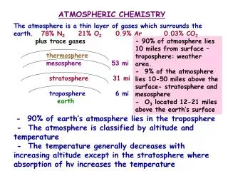
Introduction • SCISAT-1 / ACE developed by the CSA • Launched August 12, 2003 • Routine measurements began February 2004. No apparent deterioration in performance thus far. • Primary instrument is a Fourier transform spectrometer, operating between 750 and 4400 cm-1 with a resolution of 0.02 cm-1.
Retrieval Version History • Version 1.0: Initial retrievals for testing software, used to identify problems • Version 2.0: Improved the low-altitude P/T retrievals, but the VMR retrievals sometimes suffered from unphysical oscillations, and so was not widely distributed
Version History (continued) • Version 2.1: introduced an empirical function for CO2 at high altitudes during P/T retrievals (described later). Employed only for limited “analysis campaigns,” and was not applied to the entire ACE data set.
Version History (continued) • Version 2.2: Scales MSIS-calculated P and T above the highest analyzed measurement during the P/T retrieval. Previous versions simply fixed P and T in this region to MSIS values. • This version (now underway) slated as official ACE release.
P/T Retrieval process • Significant timing uncertainty for ACE-FTS measurements. We must work on a relative altitude scale rather than an absolute altitude scale. • World Geodetic System 1984 • Acceleration due to gravity: • CO2 vmr (ppm) 326.909 + 1.50155(t-to), t is time in years and to = January 1, 1977
Step 1: P and T first guess • Low altitude data (below ~ 30 km) from the Canadian Meteorological Center (CMC) • One or two day delay for analysis results rather than forecast results • High altitude data from MSIS • 40 day delay for best estimate, but one can calculate results before then with possible reduced accuracy
Step 2: First guess tangent heights • At high altitudes (taken to be above 43 km), instrument pointing information calculated from pure geometry (via STK). • Must allow for an offset (FTS FOV and suntracker axis not aligned) + timing errors • Below 43 km, refraction and clouds complicate tangent height determination. • For poor pointing knowledge, use tangent heights as parameters in P/T retrieval
Step 2 (continued) • Between 9 and ~25 km, a good first guess for altitude derived from the ratio of the baseline (Rb) at two locations (2442.6 and 2502 cm-1) in the N2/CO2 continua region Estimate density of the measurement From the CMC data, determine what altitude m corresponds to. Typically good to better than .5 km for tangent heights above 6 km.
Step 3: Establish tangent heights between 12 & 20 km • With P and T fixed to CMC data, fit for tangent heights between 12 and 20 km. These are for REGISTRATION ONLY. • Use a set of 16O12C18O lines near 2620 cm-1 • These same lines will be used later to determine tangent heights below 12 km. • Scale the strengths up by 3.5% to achieve consistency with CO2 isotopologue 1. • Physical difference between vmrs?
Step 4: First estimate for reference pressure All pressures in this region calculated from hydrostatic equilibrium and Pc. Using a reduced microwindow set, determine reference pressure Pc.
Step 5: Refine reference pressure molecules/cm3 Below 25 km:
Step 5 continued: Calculating tangent heights • Use P and T to calculate tangent height separations from the constraint of hydrostatic equilibrium [ (zc-zc+1) , (zc-zc+2)] • Propagate downwards (zc+3, zc+4, etc)
Step 5 continued: Scaling reference pressure The first calculated tangent height absorbs the effect of an error in the reference pressure Pc. Determine a refined value for Pc and fix during subsequent analysis Note: this is the result after step 6.
Step 6: Final Fitting • Fix Pc to refined value. • Redo high altitude retrieval with the full microwindow set and Pc fixed. • Redo low altitude retrieval with the new value for Pc.
Step 7: Altitude Registration • Recall that we are working on a relative altitude grid. • Compare the retrieved tangent heights to the “registration tangent heights” between 12 and 20 km determined earlier. Shift the retrieved profiles to align.
Step 8: Below 12 km • Below 12 km, we likely can’t improve upon CMC pressures and temperatures, but we need tangent heights for VMR retrievals • Fit for tangent heights using the 16O12C18O lines described previously (again scaling the line strengths by 3.5%) • Works down to 5 km or below. • Note that no seasonal or geographical variation is assumed for CO2, which is something we need to address.
Molecules being retrieved • H2O, O3, CH4, N2O, NO2, NO, HNO3, HCl, HF, CO, CFC-11, CFC-12, N2O5, ClONO2 • COF2, SF6, HCFC-22, HCN, CF4, C2H2, C2H6, OCS, CH3Cl, N2 • Testing out ClO, HOCl, H2O2, HO2NO2 • Starting on isotopologues: HDO, H218O, H217O, CH3D, 13CH4. Others to be added. • CCl4 requires line mixing. HCOOH needs interferences sorted out. H2CO.
VMR comparisons diurnal corrections for O3? MLS-ACE MLS-HALOE Implications for the chlorine budget L. Froidevaux et al, “Early Validation of Atmospheric Profiles from EOS MLS on the Aura Satellite,” IEEE Transactions on Geoscience and Remote Sensing.
Instrumental Lineshape (ILS) The nominal ILS did not fit well with the spectra. There were significant self-apodization effects beyond the normal field of view effects. Sample fitting results spanning the ACE-FTS wavenumber range
Modeling the ILS The modulation function was scaled by the factor: exp[a*x2 + b*|x|3 + c*x4] where x is optical path difference. The empirical parameters (a, b, and c) vary linearly with wavenumber. No ILS asymmetry was observed.
No apodization • Higher resolution sidelobes don’t extend as far • Inherent self-apodization effects reduce sidelobes without a need to alter the measured spectrum • Strong saturation or pressure broadening apodizes the sidelobes (resolution dependent) • In “busy” spectral regions, sidelobes tend to destructively interfere (but increase effective noise) • P/T retrieval between 60 and 90 km requires an increased extent of the ILS.
Conclusions • More data is now being collected, thanks to increased downlink capacity • Not a lot of margin now for computing power. It will take some time for version 2.2 processing to catch up.