Download
1 / 28
290 likes | 444 Views
Physical Oceanography. Basic Dynamics September 10 Conservation of Mass Newton’s Laws in the Ocean Oscillations on a Spring. Today. How do we “do” physics? Conservation of mass Newton’s Laws Statics and simple oscillations. How Do We “Do” Physics?.

E N D
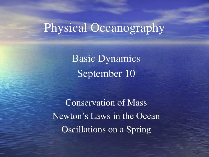
Physical Oceanography Basic Dynamics September 10 Conservation of Mass Newton’s Laws in the Ocean Oscillations on a Spring
Today How do we “do” physics? Conservation of mass Newton’s Laws Statics and simple oscillations
How Do We “Do” Physics? State variables – What do we need to specify? Pressure (p); density (); velocity (u,v,w); temperature (T); salinity (S) These are all specified as functions of position and time; e.g., p(x,y,z,t) Constraints? Conservation laws Conserve mass, momentum (counts as 3!), heat, salt. Is that enough? 7 state variables 7 constraints needed. Last one is equation of state: (x,y,z,t) = (T,S,p)
Conservation of Mass Think about cars on to and off of an island … cars = # cars in – # cars out [in a time interval (t)] Or … cars / t = # cars in / t – # cars out / t Of course, we’re not interested in the flux of cars, but the same principle applies to the flux of anything; for example, mass.
Conservation of Mass z (u)1 y z t - (u)2 y z t y z y x x Net mass flux into the volume is : m = [(u)1 - (u)2 ] y z t
An Important Aside: Taylor Series Expansions f(x) . f2 estimate df1/dx . f1 x x1 x2 = x1 + x What is our best guess at f(x2)? f2 f1 + (df1/dx) x Forms basis for numerical models of ocean and atmosphere
Back to Conservation of Mass m = [(u)1 - (u)2 ] y z t Using Taylor Series Expansion : (u)2 (u)1 + [(u)/x] x Gives : m = - [(u)/x] x y z t Now, divide by x y z t, note that V = x y z and m/ V = , and take the limit as t goes to 0, and we have : /t = - (u)/x If we treat y and z the same way, we have : /t = - [(u)/x + (v)/y + (w)/z ] or /t = - .(u)
Vector Calculus Gives the Same Result More Easily! Ignore this part if you like. But those of you who are more familiar with vector calculus may find it useful. The divergence theorem leads to: Since V can be arbitrarily small, integrands must be equal, so:
The Continuity Equation Let’s rearrange our conservation of mass statement a bit : where The final equation is how we usually write the “full” conservation of mass constraint. What does it mean? Think about air flow …
The Continuity Equation for an Incompressible Fluid What do we mean by “incompressible”? In oceanography and meteorology we mean : So, in most applications we use as an approximate statement of conservation of mass.
Newton’s Laws of Mechanics Sir Isaac Newton ( “Newtie” to his buddies ) Interesting character, to say the least. Halley story Businessman Experimentalist Theologian and Alchemist
Newton’s Laws As noted earlier, we will use conservation of momentum (remember that momentum is a vector!) to obtain 3 additional constraints on our state variables. Basically, we just apply Newton’s Laws to the fluid.
Newton’s Law of Gravitation This was Newton’s first force law. He showed that this prescription for gravity along with his laws of mechanics could explain the motions of the planets. We can recover Kepler’s Laws, in particular. This force law is written : For a mass at the surface of the Earth, we can simply to F = - mg k where g 9.8 m/s2 and k is a “unit vector” in z-direction
A Statics Problem – Mass on a Vertical Spring In statics problems we seek to determine the state of the system once it has reached a motionless equilibrium, without solving for the (often very complicated) intermediate motions. • forces = 0 z1 = L – M1g/k +k(L-z1) M1 L The spring force k(L-z1) = M1g -M1g z1
Two Masses on Two Springs +k(L-z2+z1) M2 Now we have 2 equations (one for each mass) and 2 unknowns z1 = L - g(M1+M2)/k z2 = 2L - g(M1+2M2)/k -M2g z2 +k(L-z1) M1 Force exerted by lower spring is k(L-z1) = g(M1+M2); i.e., the spring supports all the mass above it. This is a general result. -M1g -k(L-z2+z1) z1 Note: Both springs have natural length L and spring constant k.
A Simple Oscillator Now we’ll put a mass on a horizontal spring … m unstretched x = 0 F = - k x m stretched x = 0 m d2x/dt2 = -k x d2x/dt2 + (k/m) x = 0 This is a momentum equation
Finding A Solution The governing equation is : d2x/dt2 + (k/m) x = 0 We expect an oscillation, so try a solution of the form : x(t) = A cos(t) Substitute into the DE, and we find that we require that : (- 2 + k/m) A cos(t) = 0 • So, since x(t) cannot always be 0, we require that : • = (k/m)1/2 i.e., there is a “natural” frequency!
Simple Harmonic Oscillators The mass on a spring problem we just looked at is an example of what is called a “simple harmonic oscillator”. We can learn a lot about waves in general from studying these simple oscillators. Note that the dynamics of the oscillator leads to a specific, or “natural”, frequency for the oscillator. This introduces the idea of a “dispersion relation”, which is fundamental in wave problems. Note how the oscillation is maintained via a deviation from equilibrium, a restoring force towards equilibrium, an acceleration towards the equilibrium point, followed by an overshoot and a deviation from equilibrium of the opposite side sign.
Simple Harmonic Oscillators – Energetics Form an energy equation by multiplying the momentum equation by the velocity (dot product). We will do this quite often! m d2x/dt2 + k x = 0 but u = dx/dt (velocity) so u [ m du/dt + k x ] = 0 d/dt [ ½ m u2 + ½ k x2 ] = 0 d/dt [ KE + PE ] = 0 So … KE + PE = constant At equilibrium, KE is max and PE = 0; at maximum deviation, KE = 0 and PE is max. Interchange of kinetic and potential.This a very general concept!
Coupled Oscillators A pendulum is another example of a simple harmonic oscillator. But consider 2 pendula coupled together with a spring. Can you picture two distinct types of motion that this system could have? The “in phase” and “out of phase” motions represent what we call the “normal modes” of this system. Although it may not be obvious to you, it turns out that any motion that this coupled oscillator can make can be described as a linear superposition of these two modes. This is what we mean by the normal modes being “complete”.
Coordinate System • In theory, you can describe oceanic motions with a set of mathematical equations. • For equations you need a coordinate system: • Spherical for larger regions • R-H Cartesian (rectangular) for smaller regions (f-plane or Beta-plane)
N y, v z, w x, u Spherical Coordinates W x: eastward direction u: eastward velocity y: northward direction v: northward velocity z: local vertical w: vertical velocity R: vector distance from center of earth W: Earth’s rotation vector R
N y, v z, w x, u R-H Cartesian f-plane or b-plane W x: eastward direction u: eastward velocity y: northward direction v: northward velocity z: local vertical w: vertical velocity R: vector distance from center of earth W: Earth’s rotation vector R
Table 7.1 Conservation Laws Leading to Basic Equations of Fluid Motion
Ocean Circulation • Except for tides and surface gravity waves all ocean circulation is driven by difference in heating - directly – thermohaline - indirectly – heating drives winds causing wind-driven circulation
Take time to learn the names and locations of major current systems Western Boundary Currents vs. Eastern Boundary Currents
Will derive equations governing major ocean circulation patterns