Image Features
Image Features. Kenton McHenry, Ph.D. Research Scientist. Raster Images. image(234, 452) = 0.58. [ Hoiem , 2012]. Neighborhoods of Pixels. For nearby surface points most factors do not change much Local differences in brightness. [ Hoiem , 2012]. Features. Interest points


Image Features
E N D
Presentation Transcript
Image Features Kenton McHenry, Ph.D. Research Scientist
Raster Images image(234, 452) = 0.58 [Hoiem, 2012]
Neighborhoods of Pixels • For nearby surface points most factors do not change much • Local differences in brightness [Hoiem, 2012]
Features • Interest points • Points or collections of points that are somehow relevant to identifying the contents of an image • Subset of the image • Far less data than the total number of pixels • Repeatability • A feature detector should be likely to detect the feature in a scene under a variety of lighting, orientation, and other variable conditions.
Features • Edges • Corners • Blobs
Edges • Changes in intensity • Indicative of changes in albedo • Indicative of changes in orientation • Indicative of changes in distance • How do we find such regions?
Matlab • Commercial numerical computing environment • Good at matrix operations • Images are matrices • Great for quickly prototyping ideas • Image Processing Toolbox
Matlab • ls • cd Matlab • ls • whos • I = imread(‘mushrooms.jpg’); • whos • Ig = mean(I, 3); • whos • Ig • image(Ig); • colormap gray • imagesc(Ig);
Matlab • I = imread(‘intensities1.png’); • Ig = avg(I, 3); • imagesc(Ig); • surf(Ig); • axis vis3d; • rotate3d on
How do we find patterns in a Raster Image? • Geometry flashback • Vectors • 2D: (x,y) • A magnitude and direction • a = [2, 1]; • x = a(1); • y = a(2); • length = sqrt(x^2+y^2) • length = norm(a); • direction = a / norm(a); • Real numbers are called scalars (2,1)
How do we find patterns in a Raster Image? • Vector operations • With scalars: • add, subtract multiply, divide • With vectors: • cross product: gets the angle between two vectors • dot product: projects one vector into another http://en.wikipedia.org/wiki/Dot_product
How do we find patterns in a Raster Image? • a = [2,1] • b = [3,2] • a(1)*b(1) + a(2)*b(2) • dot(a,b) • dot(a/norm(a),b/norm(b)) • plot(a(1),a(2),’b.’); • plot([0,a(1)],[0,a(2)],’b-’); • hold on; • plot([0,b(1)],[0,b(2)],’r-’);
How do we find patterns in a Raster Image? • a = [2,1] • b = [-1,2] • dot(a/norm(a),b/norm(b)) • dot(a/norm(a),a/norm(a)) • b = [-2,-1] • dot(a/norm(a),b/norm(b))
How do we find patterns in a Raster Image? • Dot product gives values near 1 for similar vectors. • Not restricted to two dimensions a=[0.92,0.93,0.95,0.89] b=[0.57,0.37,0.50,0.60]
How do we find patterns in a Raster Image? • Use dot product with an image of the target • e.g. vertical edges • Use dot product at every possible location using a target:
Convolution • Given functions f(x) and g(x): • In a discrete image this is the process of calculating the dot product at every location in an image using a target image (called a filter). http://en.wikipedia.org/wiki/Convolution
Clarification: Continuous vs. Discrete • Continuous: smooth, no sharp discontinuities • Discrete: distinct separate values • Sampling: going from continuous to discrete by measuring over a small interval
Convolution • Ig = mean(imread(‘stripes1.png’), 3); • filter = [-1 1; -1 1] • imagesc(filter); • filter = filter / norm(filter); • Ig = Ig / norm(Ig); • responses = abs(conv2(Ig, filter)); • filter = [1 1; -1 -1]; • filter = filter / norm(filter); • responses = abs(conv2(Ig, filter));
So how do I get all edges? • Not so fast, we have been dealing with perfect artificial images… • Real images are noisy! • [Zoom Demo]
Noise • Ig = mean(imread(‘stripes2.png’), 3); • Ig= Ig / norm(Ig); • filter = [-1 1; -1 1] • filter = filter / norm(filter); • Ir = abs(conv2(Ig, filter)); • imagesc(Ir)
Smoothing • Assume noise is small and infrequent • Use neighbors values as a guide to remove noise
Smoothing • Ig = mean(imread(‘stripes2.png’), 3); • Ig= Ig / norm(Ig); • filter = [1 1; 1 1] • filter = filter / norm(filter); • imagesc(filter); • Ir = abs(conv2(Ig, filter)); • imagesc(Ir) • Ir = abs(conv2(Ig, filter)); • imagesc(Ir)
Smoothing • Weight so that nearby points are more important • Gaussian function http://en.wikipedia.org/wiki/Gaussian_function
Smoothing • filter = fspecial(‘guassian’, 50, 5); • filter = filter / norm(filter); • imagesc(filter); • surf(filter) • axis vis3d • rotate3d on
Smoothing • Ig = mean(imread(‘stripes2.png’), 3); • Ig= Ig / norm(Ig); • filter = fspecial(‘guassian’, 8, 2); • filter = filter / norm(filter); • Ir = abs(conv2(Ig, filter)); • imagesc(Ir) • Ir = abs(conv2(Ig, filter)); • imagesc(Ir)
Smoothing and Edges • Calculus flashback • Derivative: Rate of changes along function • Large derivatives indicate sharp changes • Edges in an image • Derivative of convolved function is equal to convolution with derivative of one of the two functions
Smoothing and Edges • Gaussian Derivative:
Smoothing and Edges • Finite differences • Approximation of derivative in discrete space • Subtract neighbors
Smoothing and Edges • 2D Guassian • Partial derivatives along x and y direction
Smoothing and Edges • gaussian = fspecial(‘guassian’, 50, 5); • guassian = filter / norm(filter); • filter = diff(gaussian, 1, 1); • imagesc(filter); • surf(filter) • axis vis3d • rotate3d on • filter = diff(gaussian, 1, 2); • imagesc(filter); • surf(filter)
Smoothing and Edges • Ig = mean(imread(‘stripes2.png’), 3); • Ig= Ig / norm(Ig); • filter = fspecial(‘guassian’, 8, 2); • filter = diff(filter, 1, 2); • filter = filter / norm(filter); • Ir = abs(conv2(Ig, filter)); • imagesc(Ir)
So now how do I get all edges? • Canny edge detector [Canny, 86] • Generate two filters one derivate in x and one in y • Convolve image with each filter • Use normalized responses in x and y direction to determine overall strength and angle • Thresholding to get strong long thin edges
Smoothing and Edges • Ig = mean(imread(‘stripes2.png’), 3); • Ig= Ig / norm(Ig); • gaussian = fspecial(‘guassian’, 8, 2); • fx = diff(gaussian, 1, 2); • fx = fx / norm(fx); • fy = diff(gaussian, 1, 1); • fy = fy / norm(fy); • Igx = abs(conv2(Ig, fx, ‘same’)); • Igy= abs(conv2(Ig, fy, ‘same’)); • imagesc(Igx) • imagesc(Igy) • imagesc(Igx + Igy); • imagesc((Igx + Igy)>100);
Edges • Ig = mean(imread(‘mushrooms.jpg’), 3); • edge(Ig, ‘canny’, 0.01); • edge(Ig, ‘canny’, 0.1); • edge(Ig, ‘canny’, 0.5);
Edges • [iPad Demo]
Lines • Hough Transform
Lines q r (x,y) = (350,200) 350 30
Lines • Threshold votes to identify lines • [Demo] http://en.wikipedia.org/wiki/Hough_transform
Lines • Notice these are infinite lines and not line segments • Extra work to find endpoints • Can be used for many parametric shapes • e.g. circles, r2 = (x2 - a2) + (y2 - b2)
Corners • Harris detector [Harris, 1988] • Partial derivatives in intensity • Averaged over a small window http://en.wikipedia.org/wiki/Corner_detection
Corners Iy Ix
Corners • [Java Demo] • [iPad Demo]
Blobs • Lets treat raster images as 2D continuous functions again • Gradient: Vector that points in the direction of greatest increase • Think intensity again • Divergence: The magnitude of changes in a vector field • In our image the vector field is the gradient calculated at every pixel • Laplacian: The divergence of a functions gradient http://homepages.inf.ed.ac.uk/rbf/HIPR2/log.htm
Why do we care about the Laplacian? • Indicates large changes in intensity when applied to an image • Edges • Ig = mean(imread(‘mushrooms.jpg’), 3); • Ig = Ig / norm(Ig); • filter = fspecial(‘log’, 8, 2); • filter = filter / norm(filter); • Ir = abs(conv2(Ig, filter)); • imagesc(Ir)
Why do we care about the Laplacian? • filter = fspecial(‘log’, 50, 5); • imagesc(filter) • surf(filter) • axis vis3d • Again not really taking Laplacian of the image but of the Gaussian function used to smooth the image http://homepages.inf.ed.ac.uk/rbf/HIPR2/log.htm
Back to blobs • Recall how convolution in discrete space involves the dot product which found vectors (i.e. patterns) that looked like the filter • The Laplacian of a Gaussian looks like a circular blob
Blobs • Ig = mean(imread(‘mushrooms.jpg’), 3); • Ig = Ig / norm(Ig); • filter = fspecial(‘log’, 100, 20); • filter = filter / norm(filter); • Ir = abs(conv2(Ig, filter)); • imagesc(Ir)
Blobs • [Java Demo]
Superpixels • Create regions of similar color (and other properties) • Graph based formulations • Treat pixels as vertices • Create edges among neighboring pixels • Weight edges by how similar the pixels they connect are