Download

1 / 33
330 likes | 442 Views
VISUALIZATION OF HYPERSPECTRAL IMAGES. ROBERTO BONCE & MINDY SCHOCKLING iMagine REU Montclair State University. Presentation Overview. Hyperspectral Images Wavelet Transform MATLAB code and results Conclusions References. Problem Statement.

E N D
VISUALIZATION OF HYPERSPECTRAL IMAGES ROBERTO BONCE & MINDY SCHOCKLING iMagine REU Montclair State University
Presentation Overview • Hyperspectral Images • Wavelet Transform • MATLAB code and results • Conclusions • References
Problem Statement • How can hyperspectral data be manipulated to enable visualization of the important information they contain?
What are hyperspectral images? • Most images contain only data in the visible spectrum • Hyperspectral images contain data from many, closely spaced wavelengths • Our camera records data from 400nm to 900nm
Hyperspectral cont. • Hyperspectral images can be thought of as being stacked on top of each other, creating an image cube • A pixel vector can be used to distinguish one material from another
Wavelets: “small waves” • Decay as distance from the center increases • Have some sense of periodicity • Can perform local analysis unlike Fourier
Wavelet Analysis and Reconstruction • Original signal is sent through high and low pass filters • Approximation: low frequency, general shape • Detail: high frequency, noise • Reconstruction involves filtering and upsampling
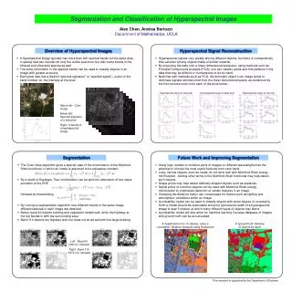
The Project • Analyzing hyperspectral signatures for image analysis can be very computationally expensive • One approach to the problem is to select a subset of the images and apply a weighting scheme to generate a useful image
Project Cont. • The plant to the right contains both real and artificial leaves • Goal: distinguish between real and artificial leaves
Last Year (2007) • Focus bands were chosen • Applied a weighting scheme • To give near infrared data more importance because the visual data is too similar • An RGB composite image is created
Last Year • Composite image to the right • They used the distance series
Preliminary results • Tried weighting, wavelet transform, different focus bands. • Results were somewhat disappointing
Procedure • Real leaves have a second peak in near-infrared region • By centering a focus band in this region, real and artificial leaves can be visualized
Results Original Image (R:60, G:30, B:20) Band-Shifted Image (R:90, G:30, B:20)
Gaussian Weighting • Similar to last approach • Choose 3 focus bands • Use Gaussian curve to do a weighted average of nearby bands • Create RGB composite image • Results are heavily dependent on what focus bands are chosen
Gaussian Weighting Figure 9 Weighted average of 3 images near bands 70, 80, and 90. The green leaves are real, the purple leaves are fake
Gaussian Weighting Figure 10 weighting using 6 images near bands 20, 30, and 40
New Approach • Instead of using 2D images from the cube, use 1D pixel vectors • Idea #1 • Choose 3 spectral vectors • Do some sort of average • Use bands corresponding to the maximum or minimum points to do an RGB composite
Idea #1 • Take the average of 3 chosen spectra, and take the 3 peaks farthest away from each other • The peaks in the diagram to the right are not very distinct
Idea #1 • Using a Gaussian curve gives more distinct peaks • The center of the Gaussian curve was the midpoint between the global maxima and global minima of all 3 pixel vectors
Idea #1 results Figure 13 real leaf, fake leaf, and pot pixel vectors chosen. Using local maxima
Idea #1 results Figure 15 Using the furthest away regional minima, rather than regional minima.
Idea #1 results Figure 16 pixel vector chosen from brick wall, plant pot, and dark rock. Used local maxima
Idea #1 results Figure 17 pixel vector chosen from brick wall, plant pot, and dark rock. Used local minima
Idea #1 results Figure 18 pixel chosen were brick, fake leaf, and rock. Used local minima.
Idea #1 results Figure 19 pixel chosen were brick, fake leaf, and rock. Used local maxima.
New Approach • Idea #2 • Choose pixels of interest • Perform wavelet decomposition • Identify coefficient positions with maxima • Perform decomposition on all pixels • Use chosen coefficients to produce a color image
Idea #2 Results • Chose 1 pixel within a real leaf and 1 pixel in brick wall for “pixels of interest” • Maxima identified for use as color values R:44 G:20 B:28
Idea #2 Results • Top: results using wavelet coefficients • Bottom: results using bands directly
Conclusions • Using wavelet coefficients could provide a superior means for visualization in some cases • Computationally expensive • More precise method for selection of pixels/peaks is needed
References: • http://www.microimages.com/getstart/pdf/hyprspec.pdf • Images from http://www.wikipedia.org/ • MATLAB help