Recursive Algorithms
Recursive Algorithms. Section 5.4. Section Summary. Recursive Algorithms Proving Recursive Algorithms Correct Recursion and Iteration ( not yet included in overheads ) Merge Sort. Recursive Algorithms.

Recursive Algorithms
E N D
Presentation Transcript
Recursive Algorithms Section 5.4
Section Summary • Recursive Algorithms • Proving Recursive Algorithms Correct • Recursion and Iteration (not yet included in overheads) • Merge Sort
Recursive Algorithms Definition: An algorithm is called recursive if it solves a problem by reducing it to an instance of the same problem with smaller input. • For the algorithm to terminate, the instance of the problem must eventually be reduced to some initial case for which the solution is known.
Recursive Factorial Algorithm Example: Give a recursive algorithm for computing n!, where n is a nonnegative integer. • Solution: Use the recursive definition of the factorial function. • procedurefactorial(n:nonnegative integer) • if n = 0then return 1 • else return n∙(n − 1) • {output is n!} Assignment: Implement this algorithm.
Recursive Exponentiation Algorithm Example: Give a recursive algorithm for computing an, where a is a nonzero real number and n is a nonnegative integer. Solution: Use the recursive definition of an. • procedurepower(a:nonzeroreal number, n:nonnegative integer) • if n = 0then return 1 • else return a∙ power (a, n − 1) • {output is an} Assignment: Implement this algorithm.
Recursive GCD Algorithm Example: Give a recursive algorithm for computing the greatest common divisor of two nonnegative integers a and b with a < b. Solution: Use the reduction gcd(a,b) = gcd(bmoda, a) and the condition gcd(0,b) = b when b > 0. • proceduregcd(a,b:nonnegative integers • with a < b) • if a = 0then return b • else return gcd(bmod a, a) • {output is gcd(a, b)} Assignment: Implement this algorithm.
Recursive Modular Exponentiation Algorithm Example: Devise a a recursive algorithm for computingbnmod m, where b, n, and m areintegers with m≥ 2, n≥ 0, and1≤b ≤ m. • Solution: (see text for full explanation) • procedurempower(b,m,n:integers with b > 0 and m≥ 2, n≥ 0) • if n = 0then • return 1 • else if nis even then • return mpower(b,n/2,m)2 mod m • else • return (mpower(b,⌊n/2⌋,m)2 mod m∙ b mod m) mod m • {output is bnmod m} Assignment: Implement this algorithm.
Recursive Binary Search Algorithm Example: Construct a recursive version of a binary search algorithm. Solution: Assume we have a1,a2,…, an, an increasing sequence of integers. Initially i is 1 and j is n. We are searching for x. • procedurebinary search(i, j, x : integers, 1≤i≤ j ≤n) • m := ⌊(i + j)/2⌋ • if x = amthen • return m • else if (x < am and i < m)then • return binary search(i,m−1,x) • else if (x > am and j >m)then • return binary search(m+1,j,x) • else return 0 • {output is location of x in a1, a2,…,anif it appears, otherwise 0} Assignment: Implement this algorithm.
Proving Recursive Algorithms Correct • Both mathematicaland str0ng induction are useful techniques to show that recursive algorithms always produce the correct output. Example: Prove that the algorithm for computing the powers of real numbers is correct. Solution: Use mathematical induction on the exponent n. BASIS STEP: a0 =1 for every nonzero real number a, and power(a,0) = 1. INDUCTIVE STEP: The inductive hypothesis is that power(a,k) = ak, for all a≠0. Assuming the inductive hypothesis, the algorithm correctly computes ak+1, since power(a,k + 1) =a∙ power (a, k) = a∙ ak =ak+1 . • procedurepower(a:nonzeroreal number, n:nonnegative integer) • if n = 0then return 1 • else return a∙ power (a, n − 1) • {output is an} −2 .
Merge Sort • Merge Sort works by iteratively splitting a list (with an even number of elements) into two sublists of equal length until each sublist has one element. • Each sublist is represented by a balanced binary tree. • At each step a pair of sublists is successively merged into a list with the elements in increasing order. The process ends when all the sublists have been merged. • The succession of merged lists is represented by a binary tree.
Merge Sort Example: Use merge sort to put the list 8,2,4,6,9,7,10, 1, 5, 3 into increasing order. Solution:
Recursive Merge Sort Example: Construct a recursive merge sort algorithm. Solution: Begin with the list of n elements L. • proceduremergesort(L = a1, a2,…,an) • if n > 1then • m := ⌊n/2⌋ • L1:= a1, a2,…,am • L2:= am+1, am+2,…,an • L:= merge(mergesort(L1), mergesort(L2)) • {L is now sorted into elements in increasing order} Assignment: Implement this algorithm. continued→
Recursive Merge Sort • Subroutine merge, which merges two sorted lists. Complexity of Merge: Two sorted lists with m elements and n elements can be merged into a sorted list using no more than m + n−1 comparisons. • procedure merge(L1, L2:sorted lists) • L := empty list • while L1 and L2 are both nonempty • remove smaller of first elements of L1 and L2 from its list; • put at the right end of L • if this removal makes one list empty • then remove all elements from the other list and append them to L • return L {L is the merged list with the elements in increasing order}
Merging Two Lists Example: Merge the two lists 2,3,5,6 and 1,4. Solution:
Complexity of Merge Sort Complexity of Merge Sort: The number of comparisons needed to merge a list with n elements is O(n log n). • For simplicity, assume that n is a power of 2, say 2m. • At the end of the splitting process, we have a binary tree with m levels, and 2m lists with one element at level m. • The merging process begins at level m with the pairs of 2m lists with one element combined into 2m−1lists of two elements. Each merger takes two one comparison. • The procedure continues , at each level (k = m, m−1,m−1,…,3,2,1) 2k lists with 2m−k elements are merged into 2k−1 lists, with 2m−k + 1 elements at level k−1. • We know (by the complexity of the merge subroutine) that each merger takes at most 2m−k + 2m−k− 1 = 2m−k+1− 1 comparisons. continued→
Complexity of Merge Sort • Summing over the number of comparisons at each level, shows that because m = log n and n = 2m. (The expression in the formula above is evaluated as 2m− 1 using the formula for the sum of the terms of a geometric progression, from Section 2.4.) • In Chapter 11, we’ll see that the fastest comparison-based sorting algorithms have O(n log n) time complexity. So, merge sort achieves the best possible big-O estimate of time complexity.


