Download
1 / 29
290 likes | 478 Views
BUSI 6480 Lecture 2. Statistics Used in One-way Analysis of Variance. Design of Experiments: A historical note. Two spoonfuls of vinegar three times a day (and 4 other treatments for scurvy) lost out to oranges and lemons in what Wikipedia credits as an "early" designed experiment. James Lind.

E N D
BUSI 6480 Lecture 2 Statistics Used in One-way Analysis of Variance
Design of Experiments: A historical note Two spoonfuls of vinegar three times a day (and 4 other treatments for scurvy) lost out to oranges and lemons in what Wikipedia credits as an "early" designed experiment. James Lind
Design of Experiments: A historical note In 1747, while serving as surgeon on HM Bark Salisbury, James Lind, the ship's surgeon, carried out a controlled experiment to develop a cure for scurvy. Lind selected 12 men from the ship, all suffering from scurvy, and divided them into six pairs, giving each group different additions to their basic diet for a period of two weeks. The treatments were all remedies that had been proposed at one time or another. They were: • A quart of cider every day • Twenty five gutts of elixir vitriol three times a day upon an empty stomach, • One half-pint of seawater every day • A mixture of garlic, mustard, and horseradish in a lump the size of a nutmeg • Two spoonfuls of vinegar three times a day • Two oranges and one lemon every day.
Design of Experiments: A historical note The men who had been given citrus fruits recovered dramatically within a week. One of them returned to duty after 6 days and the other became nurse to the rest. The others experienced some improvement, but nothing was comparable to the citrus fruits, which were proved to be substantially superior to the other treatments. In this study his subjects' cases "were as similar as I could have them", that is he provided strict entry requirements to reduce extraneous variation. The men were paired, which provided replication. From a modern perspective, the main thing that is missing is randomized allocation of subjects to treatments.
ANOVA:Testing hypothesized values of s2 • A standard assumption is that the data come from a normally distributed population. The groups are assumed to have equal population variances. • H0: s2 = s02 HA: s2s02 • H0: s2s02 HA: s2>s02 • c2 =(n-1) /s02 where is the sample variance and s02 is the hypothesized variance.
F statistic for ANOVA • Ratio of two chi-square statistics • F = (cv12 /v1)/ (cv22 / v2) where v1 and v2 are the numerator and denominator degrees of freedom. • E(F) = v2/(v2 – 2) • Thus, expected value of F is approximately one.
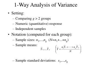
Model for One-way Anova H0: a1 = a1 = . . . = ap= 0 H1: aj 0 for some j Yij = m + aj + ei(j) where ajis a fixed effect, i = 1, . . . , n; j = 1, . . . , p Yij = + ( - ) + ( Yij - ) Score Grand Treatment Error mean effect effect = SST = SSB + SSW
Notation for Sums of Squares The letters AS represent the treatment and subject within the treatment level. The notation [AS] means to square the sum of observations within each subject treatment level. Note that there is only one observation within each subject treatment level. = [AS] The letter Y represents all observations of the dependent variable. The notation [Y] means to square the sum of all response observations and divide by the number of responses. /np = [Y] The Letter A represents all observations belonging to a level of treatment A. The notation [A] means to square the sum of Y’s within each treatment level and divide by the number of observations within each level of treatment A. /n = [A]
Sums of Squares using Symbols • SST = [AS] –[Y] • SSB = [A] – [Y] • SSW = [AS] – [A] Three terms are used in computing the sums of squares for a one-way ANOVA
Expected Values of Error Terms • E(ei(j)) = me = 0 • E( ei(j) ) = nme = 0 • E( ei(j)2 ) = nse2 • E( ei(j))2 = nse2 • E( ei(j)2) = npse2 • E( ei(j))2 = npse2
Expected Value of Mean Sum of Squares for the Fixed Effects CR-p Design • E(MSB) = se2 + • E(MSW) = se2 • E(F) ≈ E(MSB)/E(MSW) = (se2 + ) / se2 • If H0 is true and all aj = 0, then E(F) ≈ 1. What is the E(SSB)? What is the E(SSW)?
Expected Value of Mean Sum of Squares for the Random Effects CR-p Design • E(MSB) = se2 + nsa2 • E(MSW) = se2 • E(F) ≈ E(MSB)/E(MSW) = (se2 + nsa2) / se2 • If H0 is true and all sa2 = 0, then E(F) ≈ 1. • Remember for a random effects model ai is a random variable with mean 0 and variance sa2. What is the E(SSB)? What is the E(SSW)?
How do you know what ratio of sums of squares to form for the F test? • By finding the expected Mean Sum of Squares, the F statistic can be correctly computed. This will become handy as the designs become more complicated. • The expected values of the mean squares for the fixed and random effects model lead to the same ratios of mean sums of squares for the CR-p design. This will not always be true for more complex designs.
Assumptions for CR-p F Assumptions • Data come from normally distributed populations. • Observations within cells are random or at least observations are randomly assigned to cells. (Cells are determined by treatment levels.) • Numerator and denominator of F statistic are independent. • Numerator and denominator are estimates of the same population variance, se2, when H0 is true.
Model Assumptions for CR-p • The model Yij = m + aj + ei(j) contains all the sources of variation that affect Yij. • The experiment contains all the treatment levels of interest. • The error effect, ei(j) is (a) independent of other error terms, (b) normally distributed within each treatment level, ( c) mean is equal to zero, and (d) variance is constant (se2) across treatment level.
Testing for Homogeneity of Variance • H0: s12 = s22 = … = sp2
Levene Test / Brown-Forsythe Testfor testing for homogeneity of variance • Levene's test is an alternative to the Bartlett test. It is less sensitive than the Bartlett test to departures from normality. If there is strong evidence that the data do in fact come from a normal, or nearly normal distribution, then Bartlett's test has better performance. • Levene’s test: replace each observation by the absolute value of the deviation of the observation from the group mean and run a one-way ANOVA. • Brown-Forsythe test: modify Levene’s test by using the deviation of each observation from the groupmedian instead of the group mean.
HOV: Homogeneity of Variance Assume 5% significance level as the default value. If the null hypothesis is rejected use the Welch or Brown-Forsythe test ANOVA test on the means.
Transformation of the Dependent Variable to Achieve HOV or Normality – more effective with unequal group sizes.
Plotting Group Variances to Determine Transformation. Plot the variance of the group (treatment level) by the group mean (x-axis). Draw a straight line (least squares line) through the points and find the slope, b. Use p = 1- b to determine the transformation of the form:y = xp Round off p and use the closest transformation listed.
Another method for selecting the transformationUse the Smallest Range Criteria
Kruskal Wallis: Nonparametric Counterpart to the One-way ANOVA
Run the following Data using SAS and SPSS (select HOV and Welch options) one way ANOVA • /* SAS Commands ***/ • DM "Log;Clear;OUT;Clear;" ; • Data mydata; • Input Treat1 Treat2 Treat3; • datalines; • 17 18 15 • 13 12 16 • 18 26 19 • 10 18 17 • 11 9 18 • 16 30 17 • 19 12 19 • ;
Create one column of responses and another column with the grouping variable • Data Treat1; • set mydata; • resp = Treat1; • Data Treat2; • set mydata; • resp = Treat2; • Data Treat3; • set mydata; • resp = Treat3; • Data myAnovaData; • Set Treat1 Treat2 Treat3; • If _N_ <= 21 then Level = 3; • If _N_ <= 14 then Level = 2; • If _N_ <= 7 then Level = 1; • Keep resp Level; • procprint data = myAnovaData; • procexport data=myAnovaData outfile='d:MyAnovaDatainColformat.dat' dbms=dlm replace;
SAS proc to get Welch and Levine HOV test • procglm data = myAnovaData; • class Level; • model resp = Level; • means Level / hovtest welch ; • run; • quit;
SPSSOptions for the One-Way ANOVA Test for Equal Group VariancesTest for Means assuming unequal variances