Dynamic Optimization and Learning for Renewal Systems --

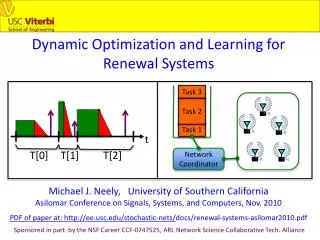
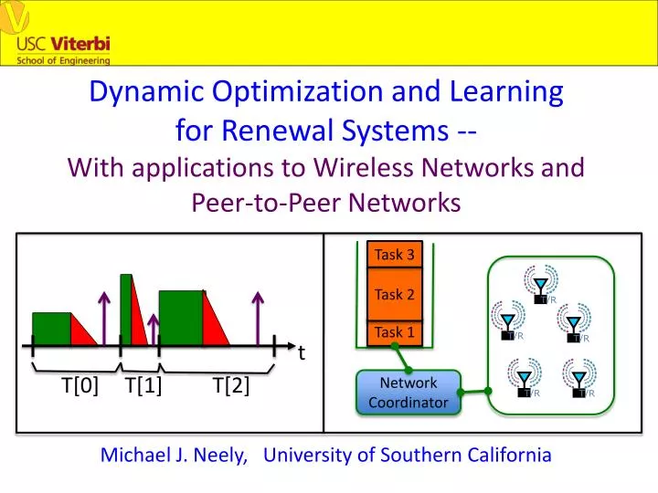
T/R T/R T/R T/R T/R Dynamic Optimization and Learning for Renewal Systems -- With applications to Wireless Networks and Peer-to-Peer Networks Task 3 Task 2 Task 1 t T[0] T[1] T[2] Network Coordinator Michael J. Neely, University of Southern California

Outline: • Optimization of Renewal Systems • Application 1: Task Processing in Wireless Networks • Quality-of-Information (ARL CTA project) • Task “deluge” problem • Application 2: Peer-to-Peer Networks • Social networks (ARL CTA project) • Internet and wireless

References: • General Theory and Application 1: • M. J. Neely, Stochastic Network Optimization with Application to Communication and Queueing Systems, Morgan & Claypool, 2010. • M. J. Neely, “Dynamic Optimization and Learning for Renewal Systems,” Proc. Asilomar Conf. on Signals, Systems, and Computers, Nov. 2010. • Application 2 (Peer-to-Peer): • M. J. Neely and L. Golubchik, “Utility Optimization for Dynamic Peer-to-Peer Networks with Tit-for-Tat Constraints,” Proc. IEEE INFOCOM, 2011. • These works are available on: • http://www-bcf.usc.edu/~mjneely/

A General Renewal System y[2] y[0] y[1] t T[0] T[1] T[2] • Renewal Frames r in {0, 1, 2, …}. • π[r] = Policy chosen on frame r. • P = Abstract policy space (π[r] in P for all r). • Policy π[r] affects frame size and penalty vector on frame r. • y[r] = [y0(π[r]), y1(π[r]), …, yL(π[r])] • T[r] = T(π[r]) = Frame Duration π[r]

A General Renewal System y[2] y[0] y[1] t T[0] T[1] T[2] • Renewal Frames r in {0, 1, 2, …}. • π[r] = Policy chosen on frame r. • P = Abstract policy space (π[r] in P for all r). • Policy π[r] affects frame size and penalty vector on frame r. • These are random functions of π[r] (distribution depends on π[r]): • y[r] = [y0(π[r]), y1(π[r]), …, yL(π[r])] • T[r] = T(π[r]) = Frame Duration π[r]

A General Renewal System y[2] y[0] y[1] t T[0] T[1] T[2] • Renewal Frames r in {0, 1, 2, …}. • π[r] = Policy chosen on frame r. • P = Abstract policy space (π[r] in P for all r). • Policy π[r] affects frame size and penalty vector on frame r. • These are random functions of π[r] (distribution depends on π[r]): • y[r] = [1.2,1.8, …, 0.4] • T[r] = 8.1 = Frame Duration π[r]

A General Renewal System y[2] y[0] y[1] t T[0] T[1] T[2] • Renewal Frames r in {0, 1, 2, …}. • π[r] = Policy chosen on frame r. • P = Abstract policy space (π[r] in P for all r). • Policy π[r] affects frame size and penalty vector on frame r. • These are random functions of π[r] (distribution depends on π[r]): • y[r] = [0.0,3.8, …, -2.0] • T[r] = 12.3 = Frame Duration π[r]

A General Renewal System y[2] y[0] y[1] t T[0] T[1] T[2] • Renewal Frames r in {0, 1, 2, …}. • π[r] = Policy chosen on frame r. • P = Abstract policy space (π[r] in P for all r). • Policy π[r] affects frame size and penalty vector on frame r. • These are random functions of π[r] (distribution depends on π[r]): • y[r] = [1.7,2.2, …, 0.9] • T[r] = 5.6 = Frame Duration π[r]

Example 1: Opportunistic Scheduling S[r] = (S1[r], S2[r], S3[r]) • All Frames = 1 Slot • S[r] = (S1[r], S2[r], S3[r]) = Channel States for Slot r • Policy π[r]: • On frame r: First observe S[r], then choose a • channel to serve (i.,e, {1, 2, 3}). • Example Objectives: thruput, energy, fairness, etc.

Example 2: Convex Programs (Deterministic Problems) Minimize: f(x1, x2, …, xN) Subject to: gk(x1, x2, …, xN) ≤ 0 for all k in {1,…, K} (x1, x2, …, xN) in A

Example 2: Convex Programs (Deterministic Problems) Minimize: f(x1, x2, …, xN) Subject to: gk(x1, x2, …, xN) ≤ 0 for all k in {1,…, K} (x1, x2, …, xN) in A Equivalent to: Minimize: f(x1[r], x2[r], …, xN[r]) Subject to: gk(x1[r], x2[r], …, xN[r]) ≤ 0 for all k in {1,…, K} (x1[r], x2[r], …, xN[r]) in A for all frames r • All Frames = 1 Slot. • Policy π[r] = (x1[r], x2[r], …, xN[r]) in A. • Time average: f(x[r]) = limR∞ (1/R)∑r=0 f(x[r]) R-1

Example 2: Convex Programs (Deterministic Problems) Minimize: f(x1, x2, …, xN) Subject to: gk(x1, x2, …, xN) ≤ 0 for all k in {1,…, K} (x1, x2, …, xN) in A Equivalent to: Minimize: f(x1[r], x2[r], …, xN[r]) Subject to: gk(x1[r], x2[r], …, xN[r]) ≤ 0 for all k in {1,…, K} (x1[r], x2[r], …, xN[r]) in A for all frames r Jensen’s Inequality: The time average of the dynamic solution (x1[r], x2[r], …, xN[r]) solves the original convex program!

Example 3: Markov Decision Problems 2 4 1 3 • M(t) = Recurrent Markov Chain (continuous or discrete) • Renewals are defined as recurrences to state 1. • T[r] = random inter-renewal frame size (frame r). • y[r] = penalties incurred over frame r. • π[r] = policy that affects transition probs over frame r. • Objective: Minimize time average of one penalty • subj. to time average constraints on others.

T/R T/R T/R T/R T/R T/R Example 4: Task Processing over Networks Task 3 Task 2 Task 1 Network Coordinator • Infinite Sequence of Tasks. • E.g.: Query sensors and/or perform computations. • Renewal Frame r = Processing Time for Frame r. • Policy Types: • Low Level: {Specify Transmission Decisions over Net} • High Level: {Backpressure1, Backpressure2, Shortest Path} • Example Objective: Maximize quality of information per unit time subject to per-node power constraints.

Quick Review of Renewal-Reward Theory (Pop Quiz Next Slide!) Define the frame-average for y0[r]: The time-average for y0[r] is then: *If i.i.d. over frames, by LLN this is the same as E{y0}/E{T}.

Pop Quiz: (10 points) • Let y0[r] = Energy Expended on frame r. • Time avg. power = (Total Energy Use)/(Total Time) • Suppose (for simplicity) behavior is i.i.d. over frames. • To minimize time average power, which one should • we minimize? (a) (b)

Two General Problem Types: 1) Minimize time average subject to time average constraints: 2) Maximize concave function φ(x1, …, xL) of time average:

Solving the Problem (Type 1): Define a “Virtual Queue” for each inequality constraint: Zl[r] clT[r] yl[r] Zl[r+1] = max[Zl[r] – clT[r] + yl[r], 0]

Lyapunov Function and “Drift-Plus-Penalty Ratio”: Z1(t) Z2(t) • Scalar measure of queue sizes: L[r] = Z1[r]2 + Z2[r]2 + … + ZL[r]2 Δ(Z[r]) = E{L[r+1] – L[r] | Z[r]} = “Frame-Based Lyap. Drift” • Algorithm Technique: Every frame r, observe Z1[r], …, ZL[r]. • Then choose a policy π[r] in P to minimize: Δ(Z[r]) + VE{y0[r]|Z[r]} E{T|Z[r]} “Drift-Plus-Penalty Ratio” =

The Algorithm Becomes: • Observe Z[r] = (Z1[r], …, ZL[r]). Choose π[r] in P to solve: • Then update virtual queues: Zl[r+1] = max[Zl[r] – clT[r] + yl[r], 0] Δ(Z[r]) + VE{y0[r]|Z[r]} E{T|Z[r]}

DPP Ratio: Theorem: Assume the constraints are feasible. Then under this algorithm, we achieve: (a) (b) Δ(Z[r]) + VE{y0[r]|Z[r]} E{T|Z[r]} For all frames r in {1, 2, 3, …}

T/R T/R T/R T/R T/R Application 1 – Task Processing: Task 3 Task 2 Task 1 Network Coordinator Idle I[r] Setup Transmit Frame r • Every Task reveals random task parameters η[r]: • η[r] = [(qual1[r], T1[r]), (qual2[r], T2[r]), …, (qual5[r], T5[r])] • Choose π[r] = [which node to transmit, how much idle] • in {1,2,3,4,5} X [0, Imax] • Transmissions incur power • We use a quality distribution that tends to be better for higher-numbered nodes. • Maximize quality/time subject to pav≤ 0.25 for all nodes.

Minimizing the Drift-Plus-Penalty Ratio: • Minimizing a pure expectation, rather than a ratio, • is typically easier (see Bertsekas, TsitsiklisNeuro-DP). • Define: • “Bisection Lemma”:

Learning via Sampling from the past: • Suppose randomness characterized by: • {η1, η2, ..., ηW} (past random samples) • Want to compute (over unknown random distribution of η): • Approximate this via W samples from the past:

Simulation: Alternative Alg. With Time Averaging Drift-Plus-Penalty Ratio Alg. With Bisection Quality of Information / Unit Time Sample Size W

T/R T/R T/R T/R T/R Concluding Sims (values for W=10): Task 3 Task 2 Task 1 Network Coordinator Idle I[r] Setup Transmit Frame r

“Application 2” – Peer-to-Peer Wireless Networking:

Network Cloud 1 2 3 5 4 • N nodes. • Each node n has download social group Gn. • Gn is a subset of {1, …, N}. • Each file f is in some subset of nodes Nf. • Each node n can request download of a file f from any node in GnNf • Transmission rates (µab(t)) between nodes are chosen in some (possibly time-varying) set G(t)

“Internet Cloud” Example 1: Uplink capacity C1uplink Network Cloud 1 2 3 5 4 • G(t) = Constant (no variation). • ∑bµnb(t) ≤ Cnuplinkfor all nodes n. • This example assumes uplink capacity is the bottleneck.

“Internet Cloud” Example 2: Network Cloud 1 2 3 5 4 • G(t) specifies a single supportable (µab(t)). • No “transmission rate decisions.” The allowable rates (µab(t)) are given to the peer-to-peer system from some underlying transport and routing protocol.

“Wireless Basestation” Example 3: = base station = wireless device • Wireless device-to-device transmission • increases capacity. • (µab(t)) chosen in G(t). • Transmissions coordinated by base station.

“Commodities” for Request Allocation • Multiple file downloads can be active. • Each file corresponds to a subset of nodes. • Queueing files according to subsets would • result in O(2N) queues. • (complexity explosion!). • Instead of that, without loss of optimality, we use the following alternative commodity structure…

“Commodities” for Request Allocation n j k m (An(t), Nn(t)) GnNn(t) • Use subset info to determine the decision set.

“Commodities” for Request Allocation n j k m (An(t), Nn(t)) GnNn(t) • Use subset info to determine the decision set. • Choose which node will help download.

“Commodities” for Request Allocation n j k m (An(t), Nn(t)) Qmn(t) • Use subset info to determine the decision set. • Choose which node will help download. • That node queues the request: • Qmn(t+1)= max[Qmn(t) + Rmn(t) - µmn(t), 0] • Subset info can now be thrown away.

Stochastic Network Optimization Problem: Maximize: ∑ngn(∑a ran) Subject to: Qmn < infinity (Queue Stability Constraint) α ∑a ran ≤ β + ∑brnb for all n (Tit-for-Tat Constraint)

Stochastic Network Optimization Problem: Maximize: ∑ngn(∑a ran) Subject to: Qmn < infinity (Queue Stability Constraint) α ∑a ran ≤ β + ∑brnb for all n (Tit-for-Tat Constraint) concave utility function

Stochastic Network Optimization Problem: Maximize: ∑ngn(∑a ran) Subject to: Qmn < infinity (Queue Stability Constraint) α ∑a ran ≤ β + ∑brnb for all n (Tit-for-Tat Constraint) concave utility function time average request rate

Stochastic Network Optimization Problem: Maximize: ∑ngn(∑a ran) Subject to: Qmn < infinity (Queue Stability Constraint) α ∑a ran ≤ β + ∑brnb for all n (Tit-for-Tat Constraint) concave utility function time average request rate α x Download rate

Stochastic Network Optimization Problem: Maximize: ∑ngn(∑a ran) Subject to: Qmn < infinity (Queue Stability Constraint) α ∑a ran ≤ β + ∑brnb for all n (Tit-for-Tat Constraint) concave utility function time average request rate β + Upload rate α x Download rate

Solution Technique for Infocom paper • Use “Drift-Plus-Penalty” framework in a new “Universal Scheduling” scenario. • We make no statistical assumptions on the stochastic processes [S(t); (An(t), Nn(t))].

Resulting Algorithm: • (Auxiliary Variables) For each n, choose an aux. variable γn(t) in interval [0, Amax] to maximize: • Vgn(γn(t)) – Hn(t)gn(t) • (Request Allocation) For each n, observe the following value for all m in {GnNn(t)}: • -Qmn(t) + Hn(t) + (Fm(t) – αFn(t)) • Give An(t) to queue m with largest non-neg value, • Drop An(t) if all above values are negative. • (Scheduling) Choose (µab(t)) in G(t) to maximize: • ∑nbµnb(t)Qnb(t)

How the Incentives Work for node n: Node n can only request downloads from others if it finds a node m with a non-negative value of: -Qmn(t) + Hn(t) + (Fm(t) – αFn(t)) Fn(t) = “Node n Reputation” (Good reputation = Low value) Fn(t) α x Receive Help(t) β+ Help Others(t)

How the Incentives Work for node n: Node n can only request downloads from others if it finds a node m with a non-negative value of: -Qmn(t) + Hn(t) + (Fm(t) – αFn(t)) Bounded Compare Reputations! Fn(t) = “Node n Reputation” (Good reputation = Low value) Fn(t) α x Receive Help(t) β+ Help Others(t)

Concluding Theorem: For any arbitrary [S(t); (An(t), Nn(t))] sample path, we guarantee: Qmn(t) ≤ Qmax = O(V) for all t, all (m,n). All Tit-for-Tat constraints are satisfied. For any T>0: liminfK∞ [AchievedUtility(KT)] ≥ liminfK∞ (1/K)∑i=1[“T-Slot-Lookahead-Utility[i]”]- BT/V K Frame 1 Frame 2 Frame 3 0 T 2T 3T

Conclusions for Peer-to-Peer Problem: • Framework for posing peer-to-peer networking as stochastic network optimization problems. • Can compute optimal solution in polynomial time. • Conclusions overall: • Renewal Optimization Framework can be viewed as “Generalized Linear Programming” • Variable Length Scheduling Modes • Many applications (task processing, peer-to-peer networks, Markov decision problems, linear programs, convex programs, stock market, smart grid, energy harvesting, and many more)

Solving the Problem (Type 2): • We reduce it to a problem with the structure of Type 1 via: • Auxiliary Variables γ[r] = (γ1[r], …, γL[r]). • The following variation on Jensen’s Inequality: • For any concave function φ(x1, .., xL) and any (arbitrarily correlated) vector of random variables • (x1, x2, …, xL, T), where T>0, we have: E{Tφ(X1, …, XL)} φ( ) E{T(X1, …, XL)} ≤ E{T} E{T}

The Algorithm (type 2) Becomes: • On frame r, observe Z[r] = (Z1[r], …, ZL[r]). • (Auxiliary Variables) • Choose γ1[r], …, γL[r] to max the below deterministic problem: • (Policy Selection) Choose π[r] in P to minimize: • Then update virtual queues: Zl[r+1] = max[Zl[r] – clT[r] + yl[r], 0], Gl[r+1] = max[Gl[r] + γl[r]T[r] - yl[r], 0]

Dynamic Optimization and Learning for Renewal Systems --