Dynamic Optimization and Learning for Renewal Systems

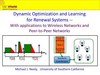
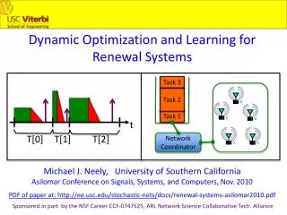
T/R T/R T/R T/R T/R Dynamic Optimization and Learning for Renewal Systems Task 3 Task 2 Task 1 t T[0] T[1] T[2] Network Coordinator Michael J. Neely, University of Southern California Asilomar Conference on Signals, Systems, and Computers, Nov. 2010 PDF of paper at: http://ee.usc.edu/stochastic-nets/docs/renewal-systems-asilomar2010.pdf Sponsored in part by the NSF Career CCF-0747525, ARL Network Science Collaborative Tech. Alliance

A General Renewal System y[2] y[0] y[1] t T[0] T[1] T[2] • Renewal Frames r in {0, 1, 2, …}. • π[r] = Policy chosen on frame r. • P = Abstract policy space (π[r] in P for all r). • Policy π[r] affects frame size and penalty vector on frame r. • y[r] = [y0(π[r]), y1(π[r]), …, yL(π[r])] • T[r] = T(π[r]) = Frame Duration π[r]

A General Renewal System y[2] y[0] y[1] t T[0] T[1] T[2] • Renewal Frames r in {0, 1, 2, …}. • π[r] = Policy chosen on frame r. • P = Abstract policy space (π[r] in P for all r). • Policy π[r] affects frame size and penalty vector on frame r. • These are random functions of π[r] (distribution depends on π[r]): • y[r] = [y0(π[r]), y1(π[r]), …, yL(π[r])] • T[r] = T(π[r]) = Frame Duration π[r]

A General Renewal System y[2] y[0] y[1] t T[0] T[1] T[2] • Renewal Frames r in {0, 1, 2, …}. • π[r] = Policy chosen on frame r. • P = Abstract policy space (π[r] in P for all r). • Policy π[r] affects frame size and penalty vector on frame r. • These are random functions of π[r] (distribution depends on π[r]): • y[r] = [1.2,1.8, …, 0.4] • T[r] = 8.1 = Frame Duration π[r]

A General Renewal System y[2] y[0] y[1] t T[0] T[1] T[2] • Renewal Frames r in {0, 1, 2, …}. • π[r] = Policy chosen on frame r. • P = Abstract policy space (π[r] in P for all r). • Policy π[r] affects frame size and penalty vector on frame r. • These are random functions of π[r] (distribution depends on π[r]): • y[r] = [0.0,3.8, …, -2.0] • T[r] = 12.3 = Frame Duration π[r]

A General Renewal System y[2] y[0] y[1] t T[0] T[1] T[2] • Renewal Frames r in {0, 1, 2, …}. • π[r] = Policy chosen on frame r. • P = Abstract policy space (π[r] in P for all r). • Policy π[r] affects frame size and penalty vector on frame r. • These are random functions of π[r] (distribution depends on π[r]): • y[r] = [1.7,2.2, …, 0.9] • T[r] = 5.6 = Frame Duration π[r]

Example 1: Opportunistic Scheduling S[r] = (S1[r], S2[r], S3[r]) • All Frames = 1 Slot • S[r] = (S1[r], S2[r], S3[r]) = Channel States for Slot r • Policy p[r]: • On frame r: First observe S[r], then choose a • channel to serve (i.,e, {1, 2, 3}). • Example Objectives: thruput, energy, fairness, etc.

Example 2: Markov Decision Problems 2 4 1 3 • M(t) = Recurrent Markov Chain (continuous or discrete) • Renewals are defined as recurrences to state 1. • T[r] = random inter-renewal frame size (frame r). • y[r] = penalties incurred over frame r. • π[r] = policy that affects transition probs over frame r. • Objective: Minimize time average of one penalty • subj. to time average constraints on others.

T/R T/R T/R T/R T/R T/R Example 3: Task Processing over Networks Task 3 Task 2 Task 1 Network Coordinator • Infinite Sequence of Tasks. • E.g.: Query sensors and/or perform computations. • Renewal Frame r = Processing Time for Frame r. • Policy Types: • Low Level: {Specify Transmission Decisions over Net} • High Level: {Backpressure1, Backpressure2, Shortest Path} • Example Objective: Maximize quality of information per unit time subject to per-node power constraints.

Quick Review of Renewal-Reward Theory (Pop Quiz Next Slide!) Define the frame-average for y0[r]: The time-average for y0[r] is then: *If i.i.d. over frames, by LLN this is the same as E{y0}/E{T}.

Pop Quiz: (10 points) • Let y0[r] = Energy Expended on frame r. • Time avg. power = (Total Energy Use)/(Total Time) • Suppose (for simplicity) behavior is i.i.d. over frames. • To minimize time average power, which one should • we minimize? (a) (b)

Two General Problem Types: 1) Minimize time average subject to time average constraints: 2) Maximize concave function φ(x1, …, xL) of time average:

Solving the Problem (Type 1): Define a “Virtual Queue” for each inequality constraint: Zl[r] clT[r] yl[r] Zl[r+1] = max[Zl[r] – clT[r] + yl[r], 0]

Lyapunov Function and “Drift-Plus-Penalty Ratio”: Z1(t) Z2(t) • Scalar measure of queue sizes: L[r] = Z1[r]2 + Z2[r]2 + … + ZL[r]2 Δ(Z[r]) = E{L[r+1] – L[r] | Z[r]} = “Frame-Based Lyap. Drift” • Algorithm Technique: Every frame r, observe Z1[r], …, ZL[r]. • Then choose a policy π[r] in P to minimize: Δ(Z[r]) + VE{y0[r]|Z[r]} E{T|Z[r]} “Drift-Plus-Penalty Ratio” =

The Algorithm Becomes: • Observe Z[r] = (Z1[r], …, ZL[r]). Choose π[r] in P to solve: • Then update virtual queues: Zl[r+1] = max[Zl[r] – clT[r] + yl[r], 0] Δ(Z[r]) + VE{y0[r]|Z[r]} E{T|Z[r]}

DPP Ratio: Theorem: Assume the constraints are feasible. Then under this algorithm, we achieve: (a) (b) Δ(Z[r]) + VE{y0[r]|Z[r]} E{T|Z[r]} For all frames r in {1, 2, 3, …}

Solving the Problem (Type 2): • We reduce it to a problem with the structure of Type 1 via: • Auxiliary Variables γ[r] = (γ1[r], …, γL[r]). • The following variation on Jensen’s Inequality: • For any concave function φ(x1, .., xL) and any (arbitrarily correlated) vector of random variables • (x1, x2, …, xL, T), where T>0, we have: E{Tφ(X1, …, XL)} φ( ) E{T(X1, …, XL)} ≤ E{T} E{T}

The Algorithm (type 2) Becomes: • On frame r, observe Z[r] = (Z1[r], …, ZL[r]). • (Auxiliary Variables) • Choose γ1[r], …, γL[r] to max the below deterministic problem: • (Policy Selection) Choose π[r] in P to minimize: • Then update virtual queues: Zl[r+1] = max[Zl[r] – clT[r] + yl[r], 0], Gl[r+1] = max[Gl[r] + γl[r]T[r] - yl[r], 0]

T/R T/R T/R T/R T/R Example Problem – Task Processing: Task 3 Task 2 Task 1 Network Coordinator Idle I[r] Setup Transmit Frame r • Every Task reveals random task parameters η[r]: • η[r] = [(qual1[r], T1[r]), (qual2[r], T2[r]), …, (qual5[r], T5[r])] • Choose π[r] = [which node to transmit, how much idle] • in {1,2,3,4,5} X [0, Imax] • Transmissions incur power • We use a quality distribution that tends to be better for higher-numbered nodes. • Maximize quality/time subject to pav≤ 0.25 for all nodes.

Minimizing the Drift-Plus-Penalty Ratio: • Minimizing a pure expectation, rather than a ratio, • is typically easier (see Bertsekas, TsitsiklisNeuro-DP). • Define: • “Bisection Lemma”:

Learning via Sampling from the past: • Suppose randomness characterized by: • {η1, η2, ..., ηW} (past random samples) • Want to compute (over unknown random distribution of η): • Approximate this via W samples from the past:

Simulation: Alternative Alg. With Time Averaging Drift-Plus-Penalty Ratio Alg. With Bisection Quality of Information / Unit Time Sample Size W

Concluding Sims (values for W=10): • Quick Advertisement: New Book: • M. J. Neely, Stochastic Network Optimization with Application to Communication and Queueing Systems. Morgan & Claypool, 2010. • http://www.morganclaypool.com/doi/abs/10.2200/S00271ED1V01Y201006CNT007 • PDF also available from “Synthesis Lecture Series” (on digital library) • Lyapunov Optimization theory (including these renewal system problems) • Detailed Examples and Problem Set Questions.

Dynamic Optimization and Learning for Renewal Systems