Download
1 / 17
560 likes | 2.04k Views
SECOND-ORDER CIRCUITS. THE BASIC CIRCUIT EQUATION. Single Loop: Use KVL. Single Node-pair: Use KCL. Differentiating. MODEL FOR RLC PARALLEL. MODEL FOR RLC SERIES. LEARNING BY DOING. THE RESPONSE EQUATION. IF THE FORCING FUNCTION IS A CONSTANT. THE HOMOGENEOUS EQUATION. LEARNING BY DOING.

E N D
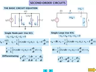
SECOND-ORDER CIRCUITS THE BASIC CIRCUIT EQUATION Single Loop: Use KVL Single Node-pair: Use KCL Differentiating
MODEL FOR RLC PARALLEL MODEL FOR RLC SERIES LEARNING BY DOING
THE RESPONSE EQUATION IF THE FORCING FUNCTION IS A CONSTANT
THE HOMOGENEOUS EQUATION LEARNING BY DOING COEFFICIENT OF SECOND DERIVATIVE MUST BE ONE DAMPING RATIO, NATURAL FREQUENCY
(modes of the system) ANALYSIS OF THE HOMOGENEOUS EQUATION Iff s is solution of the characteristic equation
DETERMINE THE GENERAL FORM OF THE SOLUTION LEARNING EXTENSIONS Divide by coefficient of second derivative Roots are real and equal Roots are complex conjugate
Form of the solution LEARNING EXTENSIONS Classify the responses for the given values of C HOMOGENEOUS EQUATION C=0.5 underdamped C=1.0 critically damped C=2.0 overdamped
THE NETWORK RESPONSE DETERMINING THE CONSTANTS
To determine the constants we need LEARNING EXAMPLE STEP 1 MODEL ANALYZE CIRCUIT AT t=0+ STEP 2 STEP 3 ROOTS STEP 4 FORM OF SOLUTION STEP 5: FIND CONSTANTS
USING MATLAB TO VISUALIZE THE RESPONSE %script6p7.m %plots the response in Example 6.7 %v(t)=2exp(-2t)+2exp(-0.5t); t>0 t=linspace(0,20,1000); v=2*exp(-2*t)+2*exp(-0.5*t); plot(t,v,'mo'), grid, xlabel('time(sec)'), ylabel('V(Volts)') title('RESPONSE OF OVERDAMPED PARALLEL RLC CIRCUIT')
LEARNING EXAMPLE NO SWITCHING OR DISCONTINUITY AT t=0. USE t=0 OR t=0+ model Form:
USING MATLAB TO VISUALIZE THE RESPONSE %script6p8.m %displays the function i(t)=exp(-3t)(4cos(4t)-2sin(4t)) % and the function vc(t)=exp(-3t)(-4cos(4t)+22sin(4t)) % use a simle algorithm to estimate display time tau=1/3; tend=10*tau; t=linspace(0,tend,350); it=exp(-3*t).*(4*cos(4*t)-2*sin(4*t)); vc=exp(-3*t).*(-4*cos(4*t)+22*sin(4*t)); plot(t,it,'ro',t,vc,'bd'),grid,xlabel('Time(s)'),ylabel('Voltage/Current') title('CURRENT AND CAPACITOR VOLTAGE') legend('CURRENT(A)','CAPACITOR VOLTAGE(V)')
LEARNING EXAMPLE KVL KCL NO SWITCHING OR DISCONTINUITY AT t=0. USE t=0 OR t=0+
USING MATLAB TO VISUALIZE RESPONSE %script6p9.m %displays the function v(t)=exp(-3t)(1+6t) tau=1/3; tend=ceil(10*tau); t=linspace(0,tend,400); vt=exp(-3*t).*(1+6*t); plot(t,vt,'rx'),grid, xlabel('Time(s)'), ylabel('Voltage(V)') title('CAPACITOR VOLTAGE')
=0 =2 LEARNING EXTENSION To find initial conditions use steady state analysis for t<0 And analyze circuit at t=0+ Once the switch opens the circuit is RLC series
To find initial conditions we use steady state analysis for t<0 KVL LEARNING EXTENSION And analyze circuit at t=0+ For t>0 the circuit is RLC series
LEARNING EXTENSION Steady state t<0 KVL Second Order Analysis at t=0+