Mixed-Layer D epth Intercomparison
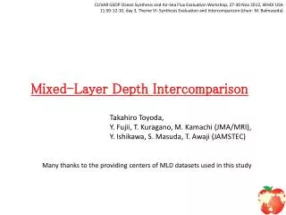
CLIVAR GSOP Ocean Synthesis and Air-Sea Fl ux E valuation Workshop, 27-30 Nov 2012, WHOI USA 11:50-12:10, day 3, Theme VI: Synthesis Evaluation and I ntercomparison (chair: M. Balmaseda ). Mixed-Layer D epth Intercomparison.

Mixed-Layer D epth Intercomparison
E N D
Presentation Transcript
CLIVAR GSOP Ocean Synthesis and Air-Sea Flux Evaluation Workshop, 27-30 Nov 2012, WHOI USA 11:50-12:10, day 3, Theme VI: Synthesis Evaluation and Intercomparison (chair: M. Balmaseda) Mixed-Layer Depth Intercomparison Takahiro Toyoda, Y. Fujii, T. Kuragano, M. Kamachi (JMA/MRI), Y. Ishikawa, S. Masuda, T. Awaji (JAMSTEC) Many thanks to the providing centers of MLD datasets used in this study
Outline • Introduction • Observational Mixed Layer Depths (MLDs) andIsothermal Layer Depths (ILDs) • Definition • Comparison of observational MLDs/ILDs • Estimate errors from time-mean and/or gridded TS • Intercomparison of MLDs/ILDs by synthesis approach • Discrepancies from Argo-based MLDs/ILDs • Scores • Possible application to climate study • North Pacific • North Atlantic • Barrier Layers in the equatorial Indo-Pacific • Summary and discussion
Importance of MLD analysis • MLD characterizes heatand fresh-water cycle in the ocean surface layer. • Surface water masses are generated in ML, followed by subduction to the ventilated thermocline layer and thereby forming physical properties in subsurface layer (e.g., T, S, PV). • Important element of the bio-geochemical cycle (e.g., CO2; lower figure) • Accurate description of MLD distribution required for better understanding of climate variabilities and prediction. Annual sea-air CO2 flux from Takahashi (1997; updated) Ocean uptake in deep ML regions is clearly seen.
Syntheses representing interannual variability in the global ocean • Improvement in modeling and assimilation techniques and increase of observations offer a better description of global ocean processes. • Evaluation of global ocean syntheses is needed in the context of observation-based estimates. • MLD is one of the most important metrics for the dynamical process of climate variation. • Intercomparison of the seasonal to interannualvariabilities in MLDs on global scales will provide useful information to the assimilation community and the user community (e.g., in CLIVAR) to further activate both the synthesis approach and the study of climate variabilityand predictability. • Assimilation community can apply the syntheses to the climate study firstly, since this would be followed by other users and then more robust evaluation would be done from various aspects.
Datasets • [16 ocean sysntheses submitted] • GLORYS2V1 (Mercator): 3DVAR, 1/4 deg, 50 levs, 1993-2009 • PSY3V3 (Mercator): operational best estimate of GLORYS2V1, 2009-2011 • C-GLORS (CMCC): 3DVAR, 1/4 deg, 50 levs, 2000-2010 • UR025.4 (Univ. Reading): ensemble OI, 1/4 deg, 46 levs, 1993-2010 • ORAS4 (ECMWF): 3DVAR+FGAT, 1x(0.3-1) deg, 42levs, 1958-2011 • GECCO2 (Univ. Hamburg): 4DVAR, 1x(1/3-1) deg, 50 levs, 1948-2011.11 • GEOS5 (GMAO): ensemble OI, 1/2x(1/4-1/2) deg, 40 levs, 1993-2011 • ECCO (JPL): Kalmanfilter and RTS smoother, 1x(0.3-1) deg, 46 levs, 1993-2011 • ECDA3 (GFDL): coupled EnKF, 1x(0.3-1) deg, 50 levs, 2005-2011 • K7-ODA (JAMSTEC): 4DVAR, 1 deg (75S-80N), 45 levs, 1975-2009 • MOVE-G2 (MRI): 3DVAR+FGAT, 1x(0.3-0.5) deg, 53 levs, 1979-2011 • MOVE-CORE (MRI): 3DVAR+FGAT, 1x0.5 deg, 51 levs, 1948-2007 • MOVE-C (MRI): 3DVAR, coupled model, 1x(0.3-1) deg (75S-75N), 50 levs, 1950-2011 • K7-CDA (JAMSTEC): coupled 4DVAR, 1 deg, 45 levs, 2000-2007.3 • EN3v2a (UKMO): no model, OI, 1 deg, 2005-2011 • ARMOR-3D (CLS): no model, OI, 1/3 deg (82S-82N), 24 levs (0-1500m), 1993-2010 • [Additional MLD datasets for references] (with no model) • MILA_GPV (JAMSTEC): based on Argoprofiles,2x2 deg, 2001-2011 • de Boyer Montegut et al. (2004)based on TSprofiles (1941-2008), 2x2 deg, climatology • NODC MLD: from WOA(98) TS, climatology
Definitions of MLDs and ILDs • Based on monthly TS. • MLDs and ILDs are defined as • MLDr003m: σθ(z=MLD)-σθ(z=10m)=Δρ, Δρ=0.03 kg m-3 • MLDr0125m: Δρ=0.125 kg m-3 • ILDt02m: |T(z=ILD)-T(z=10m)|=ΔT, ΔT=0.2˚C • ILDt05m: ΔT=0.5˚C • Interannual-mean (2001-2011 average) values are calculated monthly (or shorter period depending on length of each synthesis). • Mainly referred to MILA_GPV (JAMSTEC) based on individualTSprofiles from Argo floats: one of the most realistic datasets for MLD/ILD in our analysis.
Intercomparison between observational MLDs EN3v2a (UKMO),ARMOR-3D (CLS): based on monthly-meanTS(time-series) MILA_GPV (JAMSTEC), de Boyer Montegut et al. (2004): based on individual TS profiles NODC MLD: from WOA98 (monthly climatological TS) Profiles→MLDs→gridded MLDs MLD (0.03 kg m-3 criterion) in March MILA_GPV (JAMSTEC) Difference from MILA_GPV de Boyer Montegut EN3v2a (UKMO) ARMOR-3D (CLS) [m] [m] Zonal-mean RMSD • MLDs derived from monthly-meangriddedTS are shallower than those from TS profiles (10-20 m shallower in low latitude and much more in mid-high latitudes) • Consistent with previous studiess (de Boyer Montegutet al.) • MLD Differences can be attributed to the differences in1) Vertical resolution between observations and datasets2) Instantaneous and mean TS profiles3) Observational data4) The number of observations ↔ horizontal smoothing EN3v2a(UKMO) de BoyerMontegut NODC Argo ARMOR-3D(CLS) MLDr0125 MLDr003 [m]
Effects of vertical resolution case (2-2) case (1) MLD case (2-1) (real MLD) MLD grid • Assume the above 3 cases: high resolution case (1) and low resolution cases (2). • MLD is estimated realistically in high resolution case (1) and low resolution case (2-1). • But in the low resolution case (2-2), MLD is underestimated. • This skewness of biases in the low resolution cases is due to the fact that density change in thermocline is often much larger than Δρ of MLD criterion as shown above. • On average, MLD is underestimated when using the low-resolution gridded data (e.g., syntheses)
Effects of time-mean and criterion • In addition to MLDs/ILDs based on monthly TS (e.g., MLDr003m), MLDs/ILDs are calculated from on-line snapshot TS data in the MOVE-G2 experiment (e.g., MLDr003i). • MLDs/ILDs from Interannually-averaged monthly TS (e.g., MLDr003y) are also compared. • Dr. Fabrice Hernandez kindly provided MLDs/ILDs derived from daily TS(e.g., MLDr003d), which are compared with MLDs/ILDs frommonthly TSdata of GLORYS2V1 (Mercator). [from MOVE-G2 (MRI)] MLDr003m-i MLDr0125m-i • Underestimation in case of time-mean TS. • Re-stratification in early spring as well as sudden deepening in early winter likely increases errors. Annual march of zonal-mean RMSE [MRI] ivsmivsy [Mercator] dvsm [form GLORYS2V1 (Mercator)] MLDr003m-d MLDr0125m-d (MLDr003) 40˚N 70˚S Longer time-mean ↓ Larger error [m] Larger criterion → Smaller error
More errors in ILDs from time-mean temperature • For ILDs, large errors occur in the subpolar regions associated with the weak mesothermalstructurepeculier to the subarctic/subpolar regions. ILDt05m-i (MOVE-G2) Example from MOVE-G2: TS at (180˚, 70˚S) during Jan-Jun 2001 c.i.=0.05psu c.i.=0.3˚C Gridded monthly ILDt05m-d (GLORYS2V1) [m] S T T January June • Too deep ILD is estimated during one month from this time-series when gridded monthly. [˚C]
Intercomparison with reference to Argo MLDs • Differences from MILA_GPV (JAMSTEC)based on Argo TS profiles are shown. • Note that smaller biases do not necessarily indicate a better synthesis, because (1) there exist shallow biases due to the use of monthly-mean and gridded (with lower vertical resolution than observations) TS instead of individual profilesand(2) using Argo data in syntheses, difference between products is more reduced by the stronger restoring to observations.
MLDr0125m difference from MILA_GPV (JAMSTEC) in February [m]
MLDr0125m difference from MILA_GPV (JAMSTEC) in February 1 1/3 1/4 1/4 No model OI No model OI ERA-I SEEK ERA SEEK 1/4 1/4 1 1 Surface flux ERA-I OI ERA-I OI ERA 3DVAR (NCEP1) 4DVAR 1/2 1 1 1 Surface flux Surface flux GMAO OI (NCEP) KF+RTS Coupled EnKF (NCEP2) 4DVAR 1/2 1/2 1 1 Surface flux JRA 3DVAR CORE 3DVAR (Coupled) 3DVAR Coupled 4DVAR [m]
NPESTMW, NPTW Barrier layer thickness comparison Defined here as: BLT=ILDt05m-MLDr0125m ITCZ OBS ICW SPESTMW SPCZ [m] • BLs are thin in the smoother approach while thick in the coupled case (K7-CDA). • Correction of ERA-I based on GEWEX in GLORYS2V1 and C-GLORS likely thickens BLs. • Reproductions of BLs related to salty waters from subtropics are similar in each synthesis. 10
Scores on time-mean values • RMSDs of interannual-mean monthly MLDs/ILDs between MILA_GPV and syntheses. • ILDs are compared within 40˚S-40˚N, because of large biases toward high latitudes. • Shaded dark (light) orange indicates values less than mean by 1-σor smallest (0.5-σ). • Right 4 columns are for RMSDs of seasonal variation defined here as maximum minus minimum values in each grid point. RMSDs of monthly values RMSD of Seasonal variation [m]
RMSDs from other datasets RMSDs from de Boyer Montegut Seasonal variation RMSDs from NODC MLD Seasonal variation • Comparison of syntheses with no model indicates that ARMOR-3D is closer to MILA_GPV and de Boyer Montegut et al. (2004) whereas EN3v2a is closer to NODC MLD, which might be due to the resolutions.
Regional RMSDs from MILA_GPV North Pacific (>20˚N) North Atlantic (>20˚N) Tropics (20˚S-20˚N) Southern Hemisphere (<20˚S)
Interannual anomalies • MILA_GPV provides monthly MLDs/ILDs from Jan 2001. • Coverage (with 2x2 deg grid) is small and distribution is fluctuated in early years. Jan2001 Dec2004 Dec2011 [m] Dec2004 • For MLDs, results from CORE forcing (MOVE-CORE) and coupled case (ECDA3 and MOVE-C) look fine. • For ILDs, correction based on GEWEX works better on ERA-I (GLORYS2V1 and C-GLORS). RMSDs of interannualanomaliy from MILA_GPV
Use for climate studies • Datasets taking temporal and spatial coverage has the importantimplication to climate studies. • Ensemble-mean monthly time-seriesduring 1948-2011 are calculated from all submitted syntheses. • Time-series of annual maxima of MLDs/ILDs are constructed for the analysis in mid-latitudes, since annual maxima are dynamically important and contain integrated thermodynamical processes from surface cooling in whole winter although the timing when they occur differs among syntheses. Histogram of annual maxima of MLDr0125mfrom all syntheses • Maxima during January-April in the Northern Hemisphere and during July-October in the Southern Hemisphere are used in the following analysis.
Explained variance by the ensemble mean • An interannualvariance derived from all datasets is defined here at each grid point as mld: MLD/ILD from each synthesis overbar: monthly average over 2001-2011 mldens: ensemble mean MLD/ILD “r” for annual maxima of MLDr0125m Large values of “r” indicates consistent interannual variability among syntheses. inconsistent consistent
“r” in the North Pacific EOF analysis in the North Pacific • An EOF analysis is performed for the ensemble-mean annual-maximum MLDr0125m field during 2001-2011 in the region with r>0.3 in the North Pacific. • Time-series and pattern of each principal component are projected in the remnant regions and to the period before 2000, respectively. • The 1st & 2nd principal components seem to be related to PDO and Mode Waters. • These are discussed in the following slides. • The 3rd and higher modes are confined on smaller scales. [m] EOF #1 (40%) [˚C] EOF #2 (21%) (Contours denote the mean MLD.) Pacific Decadal Oscillation (PDO) defined as the leading EOF of winter SST anomalies in the Pacific Ocean (>20˚N).Patterns of SST (color), SLP (contour), and wind (arrow) anomalies from Mantua et al. (1997). EOF #3 (7%)
Comparison of time-series EOF #2 PDO(-) (135˚E-160˚E, 30˚N-35˚N) Subtropical Mode Water EOF1 [˚C] 20 Projection of EOF map during 1948-2000. 15 EOF analysis EOF2×20 ensemble mean EOF1×(-40) -STMW temp from JMA obs along 137˚E 0m (180˚-160˚W, 30˚N-40˚N) Central Mode Water -EOF1×factor -each member-ensemble mean EOF #1 0m (140˚W-130˚W, 25˚N-30˚N) Eastern Subtropical Mode Water EOF1×20
“r” in the North Atlantic EOF analysis in the North Atlantic Leading principal component (56%) of the MLD variability in the North Atlantic (>20N; r>0.3) during 2001-2011 [m] EOF analysis Projection NAO(-) Positive NAO from NOAA/Lamont-Doherty Earth Observatory NAO pamphlet • MLD variability in the STMW & SPMW formation regions related to North Atlantic Oscillation (NAO). • Consistent with previous study (Joice et al., 2000). • “r” is not so large in the Norwegian Sea but EOF1 map is similar to the tri-polar distribution of SSTA in the North Atlantic (Tanimono and Xie, 2002). EOF1
Barrier layer in the equatorial Indo-Pacific [m] X axis: 40˚E-80˚W Y axis: 1993-2011 - + Nino3.4 - +
Summary and discussion We have performed the intercomparison of MLDs/ILDs from syntheses with various models, resolutions, forcings, and assimilation methods. Syntheses have an advantage in their spacio-temporal coverage. The ensemble of synthesis datasets would enhance our understanding of interannual MLD variability, at least in open oceans where a similar variability is seen among syntheses. Our result could be more discussed in connection with other intercomparisons presented in this WS. More observations or maintenance of current observations are of great value for analysis/synthesis of the global MLD variability. Comparison with regional assimilation results with higher resolution might be more beneficial. A variety of syntheses (e.g., with a σ-model) would strengthen the robustness of the ensemble approach.
Acknowledgements • To Dr. Fabrice Hernandez in the Mercator Ocean and many providers of MLD/ILD data. • The MLD and ILD data based on Argo profiling float data (Hosoda et al., 2010) which we used in this study are provided by the Research Institute for Global Change, Japan Agency for Marine-Earth Science and Technology.