Download
1 / 17
170 likes | 280 Views
An Image Filtering Technique for SPIDER Visible Tomography. N. Fonnesu M. Agostini, M. Brombin, R.Pasqualotto, G.Serianni. 3rd PhD Event- York- 24th-26th June 2013. Introduction.

E N D
An Image Filtering Technique for SPIDER Visible Tomography N. Fonnesu M. Agostini, M. Brombin, R.Pasqualotto, G.Serianni 3rd PhD Event- York- 24th-26th June 2013
Introduction The ITER Heating Neutral Beam (HNB) injector, based on negative ions accelerated at 1MV, will be tested and optimized in the SPIDER source and MITICA full injector prototypes, using a set of diagnostics not available on the ITER HNB. SPIDER (Full size prototype of the HNB source, ions accelerated at 100 kV) MITICA (Full size prototype of the HNB, ions accelerated at 1 MV) • My research activity is focused on: • Optical diagnostics for Neutral Beam (i.e. tomography) • Analyses and numerical models dedicated to characterize the ion extraction from the source, beam optics in the accelerator and beam transport in the injector • Fast neutron measurements on RFX (Reversed field pinch device) 3rd PhD Event- York- 24th-26th June 2013 – Nicola Fonnesu
Outline • Tomography: • what is it? • why is it important in SPIDER ? • tomography code and inversion technique • The role of instrumental noise in tomography reconstructions • Filtering technique in the spatial domain and results • Conclusions and future works 3rd PhD Event- York- 24th-26th June 2013 – Nicola Fonnesu
What is tomography? Tomography is the reconstruction of a cross-section (or a slice) of an object from its projections (i.e. integral of the image at a given angle). Fan of LoSs Fan of LoSs SPIDER beam (currentof H/D ions accelerated at 100 kV) Fan of LoS Every projection is made of a large number of lines of sight (LoSs) 3rd PhD Event- York- 24th-26th June 2013 – Nicola Fonnesu
beam source lens viewport CCD Diagnostic room PC PC E/O PC O/E SPIDER Visible Tomography Main target: measurement of the beam uniformity with sufficient spatial resolution and of its evolution throughout the pulse duration. Observing the emission of Hα (Dα) radiation (due to collisions between background gas and ions) on a plane perpendicular to the beam with a set of 3127 lines-of-sight, will allow a tomographic reconstruction of the two dimensional beam emission function, which is proportional to the beam density. The maximum acceptable deviation from beam uniformity is ±10% the deviation of the reconstruction from the real emissivity of the beam has to be sufficiently lower than this value 3rd PhD Event- York- 24th-26th June 2013 – Nicola Fonnesu
Inversion technique: the pixel method j-th line of sight Integrated Hα (Dα) radiation along the j-th line of sight Emissivity of the beam From the line integrated measurements we want to obtain the 2D map of the beam emission PIXEL METHOD Ij : line-integrated signal of the line j εi: emissivity of the pixel i ai,j: fraction of area of pixel i observed by line j The unknowns are the emittivities εi of each pixel i of the image which can be obtained by inverting the matrix a Pixel i 1280 beamlets divided into 16 beamlet groups SART METHOD 3rd PhD Event- York- 24th-26th June 2013 – Nicola Fonnesu
Instrumental noise in the line integrated signals Phantoms (i.e. 2D emissivity profiles) that reproduce different experimental beam configurations (non-uniformity of ±10%, uniform profile, two beamlet groups turned off) are simulated and reconstructed by the tomography code with satisfactory results. ±10% Reference phantom …adding a random noise (unif. distr., max 20%) However, if we simulate noisy input data, errors in the reconstructed image shows that noise acts as a limiting factor for the maximum achievable resolution. 3rd PhD Event- York- 24th-26th June 2013 – Nicola Fonnesu
Errors in the reconstructed beam profile npix 3rd PhD Event- York- 24th-26th June 2013 – Nicola Fonnesu
Filtering in the spatial domain The filtering algorithm is based on Lee’s formula [1] that allows to calculate the estimated noise-free pixel intensity just considering its neighborhood: this value will represent the filtered intensity for the corresponding pixel. Pixel’s neighborhood is defined by a squared window (5x5 pixels gives better results) Pixel i,j filtered value of the pixel i,j at the step l+1 value of the pixel i,j at the step l parameter (variance,mean of the pixel’s neighborhood) local average pixel’s value at the step l [1] J.S. Lee, Optical Engineering 25 (5), 636-646 (1986) 3rd PhD Event- York- 24th-26th June 2013 – Nicola Fonnesu
Filtering in the spatial domain • In order to minimize the reconstruction errors, the algorithm applies iteratively the Lee’s formula. 3rd PhD Event- York- 24th-26th June 2013 – Nicola Fonnesu
Filteredreconstructions: linearemissivityvariation 3rd PhD Event- York- 24th-26th June 2013 – Nicola Fonnesu
Filteredreconstructions: constantemissivity 3rd PhD Event- York- 24th-26th June 2013 – Nicola Fonnesu
Filteredreconstructions: 2 beamletgroups off The algorithm tends to smooth the boundary of the zero-emissivity area present in the case a beamlet group is switched off, affecting the entire profile. It is necessary to introduce a delta function that allows not to consider pixels with quasi-zero emissivity in the local statistics (for the calculation of the mean of x and k parameter). 3rd PhD Event- York- 24th-26th June 2013 – Nicola Fonnesu
Comparisonwith a low pass filter Lee’s filter FFT+ Low Pass (Hann) filter 3rd PhD Event- York- 24th-26th June 2013 – Nicola Fonnesu
Conclusions • The maximum errors (in reconstructions with 640 pixels) are reduced to values up to 3.5% considering different operating conditions of SPIDER. • Filtering in the spatial frequency domain could give similar results (for the same level of noise) just considering a lower number of pixels (i.e. 32 or 64). • A higher number of pixels can go beyond the simple detection of the lack of uniformity of the beam, giving information about its causes and suggesting possible solutions. • Encouraging attempt to demonstrate the feasibility to suppress instrumental noise by a post-processing algorithm that does not increase significantly the processing time. 3rd PhD Event- York- 24th-26th June 2013 – Nicola Fonnesu
Future Works • Filtering algorithm for MITICA visible tomography • Development of the tomography code for N1O (60 kV negative ion source) 3rd PhD Event- York- 24th-26th June 2013 – Nicola Fonnesu
THANK YOU FOR YOUR ATTENTION ! 3rd PhD Event- York- 24th-26th June 2013 – Nicola Fonnesu