Algorithm Analysis
470 likes | 685 Views
Algorithm Analysis. Introduction. Data structures Methods of organizing data What is Algorithm? a clearly specified set of simple instructions on the data to be followed to solve a problem Takes a set of values, as input and produces a value, or set of values, as output

Algorithm Analysis
E N D
Presentation Transcript
Introduction • Data structures • Methods of organizing data • What is Algorithm? • a clearly specified set of simple instructions on the data to be followed to solve a problem • Takes a set of values, as input and • produces a value, or set of values, as output • May be specified • In English • As a computer program • As a pseudo-code • Program = data structures + algorithms
Introduction • Why need algorithm analysis ? • writing a working program is not good enough • The program may be inefficient! • If the program is run on a large data set, then the running time becomes an issue
Example: Selection Problem • Given a list of N numbers, determine the kth largest, where k N. • Algorithm 1: (1) Read N numbers into an array (2) Sort the array in decreasing order by some simple algorithm (3) Return the element in position k
Algorithm 2: (1) Read the first k elements into an array and sort them in decreasing order (2) Each remaining element is read one by one • If smaller than the kth element, then it is ignored • Otherwise, it is placed in its correct spot in the array, bumping one element out of the array. (3) The element in the kth position is returned as the answer.
Which algorithm is better when • N =100 and k = 100? • N =100 and k = 1? • What happens when • N = 1,000,000 and k = 500,000? • We come back after sorting analysis, and there exist better algorithms
Algorithm Analysis • We only analyze correct algorithms • An algorithm is correct • If, for every input instance, it halts with the correct output • Incorrect algorithms • Might not halt at all on some input instances • Might halt with other than the desired answer • Analyzing an algorithm • Predicting the resources that the algorithm requires • Resources include • Memory • Communication bandwidth • Computational time (usually most important)
Factors affecting the running time • computer • compiler • algorithm used • input to the algorithm • The content of the input affects the running time • typically, the input size (number of items in the input) is the main consideration • E.g. sorting problem the number of items to be sorted • E.g. multiply two matrices together the total number of elements in the two matrices • Machine model assumed • Instructions are executed one after another, with no concurrent operations Not parallel computers
Different approaches • Empirical: run an implemented system on real-world data. Notion of benchmarks. • Simulational: run an implemented system on simulated data. • Analytical: use theoretic-model data with a theoretical model system. We do this in 171!
Example • Calculate • Lines 1 and 4 count for one unit each • Line 3: executed N times, each time four units • Line 2: (1 for initialization, N+1 for all the tests, N for all the increments) total 2N + 2 • total cost: 6N + 4 O(N) 1 2N+2 4N 1 1 2 3 4
Worst- / average- / best-case • Worst-case running time of an algorithm • The longest running time for any input of size n • An upper bound on the running time for any input guarantee that the algorithm will never take longer • Example: Sort a set of numbers in increasing order; and the data is in decreasing order • The worst case can occur fairly often • E.g. in searching a database for a particular piece of information • Best-case running time • sort a set of numbers in increasing order; and the data is already in increasing order • Average-case running time • May be difficult to define what “average” means
Running-time of algorithms • Bounds are for the algorithms, rather than programs • programs are just implementations of an algorithm, and almost always the details of the program do not affect the bounds • Algorithms are often written in pseudo-codes • We use ‘almost’ something like C++. • Bounds are for algorithms, rather than problems • A problem can be solved with several algorithms, some are more efficient than others
Growth Rate • The idea is to establish a relative order among functions for large n • c , n0 > 0 such that f(N) c g(N) when N n0 • f(N) grows no faster than g(N) for “large” N
Growth rates … • Doubling the input size • f(N) = c f(2N) = f(N) = c • f(N) = log N f(2N) = f(N) + log 2 • f(N) = N f(2N) = 2 f(N) • f(N) = N2 f(2N) = 4 f(N) • f(N) = N3 f(2N) = 8 f(N) • f(N) = 2N f(2N) = f2(N) • Advantages of algorithm analysis • To eliminate bad algorithms early • pinpoints the bottlenecks, which are worth coding carefully
Asymptotic notations • Upper bound O(g(N) • Lower bound (g(N)) • Tight bound (g(N))
Asymptotic upper bound: Big-Oh • f(N) = O(g(N)) • There are positive constants c and n0 such that f(N) c g(N) when N n0 • The growth rate of f(N) is less than or equal to the growth rate of g(N) • g(N) is an upper bound on f(N)
In calculus: the errors are of order Delta x, we write E = O(Delta x). This means that E <= C Delta x. • O(*) is a set, f is an element, so f=O(*) is f in O(*) • 2N^2+O(N) is equivelent to 2N^2+f(N) and f(N) in O(N).
Big-Oh: example • Let f(N) = 2N2. Then • f(N) = O(N4) • f(N) = O(N3) • f(N) = O(N2) (best answer, asymptotically tight) • O(N2): reads “order N-squared” or “Big-Oh N-squared”
Some rules for big-oh • Ignore the lower order terms • Ignore the coefficients of the highest-order term • No need to specify the base of logarithm • Changing the base from one constant to another changes the value of the logarithm by only a constant factor If T1(N) = O(f(N) and T2(N) = O(g(N)), • T1(N) + T2(N) = max( O(f(N)), O(g(N)) ), • T1(N) * T2(N) = O( f(N) * g(N) )
Big Oh: more examples • N2 / 2 – 3N = O(N2) • 1 + 4N = O(N) • 7N2 + 10N + 3 = O(N2) = O(N3) • log10 N = log2 N / log2 10 = O(log2 N) = O(log N) • sin N = O(1); 10 = O(1), 1010 = O(1) • log N + N = O(N) • logk N = O(N) for any constant k • N = O(2N), but 2N is not O(N) • 210N is not O(2N)
lower bound • c , n0 > 0 such that f(N) c g(N) when N n0 • f(N) grows no slower than g(N) for “large” N
Asymptotic lower bound: Big-Omega • f(N) = (g(N)) • There are positive constants c and n0 such that f(N) c g(N) when N n0 • The growth rate of f(N) is greater than or equal to the growth rate of g(N). • g(N) is a lower bound on f(N).
Big-Omega: examples • Let f(N) = 2N2. Then • f(N) = (N) • f(N) = (N2) (best answer)
tight bound • the growth rate of f(N) is the same as the growth rate of g(N)
Asymptotically tight bound: Big-Theta • f(N) = (g(N)) iff f(N) = O(g(N)) and f(N) = (g(N)) • The growth rate of f(N) equals the growth rate of g(N) • Big-Theta means the bound is the tightest possible. • Example: Let f(N)=N2 , g(N)=2N2 • Since f(N) = O(g(N)) and f(N) = (g(N)), thus f(N) = (g(N)).
Some rules • If T(N) is a polynomial of degree k, then T(N) = (Nk). • For logarithmic functions, T(logm N) = (log N).
General Rules • Loops • at most the running time of the statements inside the for-loop (including tests) times the number of iterations. • O(N) • Nested loops • the running time of the statement multiplied by the product of the sizes of all the for-loops. • O(N2)
Consecutive statements • These just add • O(N) + O(N2) = O(N2) • Conditional: If S1 else S2 • never more than the running time of the test plus the larger of the running times of S1 and S2. • O(1)
Using L' Hopital's rule This is rarely used in 171, as we know the relative growth rates of most of functions used in 171! • ‘rate’ is the first derivative • L' Hopital's rule • If and then = • Determine the relative growth rates (using L' Hopital's rule if necessary) • compute • if 0: f(N) = o(g(N)) and f(N) is not (g(N)) • if constant 0: f(N) = (g(N)) • if : f(N) = (f(N)) and f(N) is not (g(N)) • limit oscillates: no relation
Our first example: search of an ordered array • Linear search and binary search • Upper bound, lower bound and tight bound
Linear search: // Given an array of ‘size’ in increasing order, find ‘x’ int linearsearch(int* a[], int size,int x) { int low=0, high=size-1; for (int i=0; i<size;i++) if (a[i]==x) return i; return -1; } O(N)
Iterative binary search: int bsearch(int* a[],int size,int x) { int low=0, high=size-1; while (low<=higt) { int mid=(low+high)/2; if (a[mid]<x) low=mid+1; else if (x<a[mid]) high=mid-1; else return mid; } return -1 }
Iterative binary search: int bsearch(int* a[],int size,int x) { int low=0, high=size-1; while (low<=higt) { int mid=(low+high)/2; if (a[mid]<x) low=mid+1; else if (x<a[mid]) high=mid-1; else return mid; } return -1 } n=high-low n_i+1 <= n_i / 2 i.e. n_i <= (N-1)/2^{i-1} N stops at 1 or below there are at most 1+k iterations, where k is the smallest such that (N-1)/2^{k-1} <= 1 so k is at most 2+log(N-1) O(log N)
Recursive binary search: int bsearch(int* a[],int low, int high, int x) { if (low>high) return -1; else int mid=(low+high)/2; if (x=a[mid]) return mid; else if(a[mid]<x) bsearch(a,mid+1,high,x); else bsearch(a,low,mid-1); } O(1) O(1) T(N/2)
Solving the recurrence: • With 2k = N (or asymptotically), k=log N, we have • Thus, the running time is O(log N)
Lower bound, usually harder than upper bound to prove, informally, find one input example , that input has to do ‘at least’ an amount of work that amount is a lower bound • Consider a sequence of 0, 1, 2, …, N-1, and search for 0 • At least log N steps if N = 2^k • An input of size n must take at least log N steps • So the lower bound is Omega(log N) • So the bound is tight, Theta(log N)
Another Example • Maximum Subsequence Sum Problem • Given (possibly negative) integers A1, A2, ...., An, find the maximum value of • For convenience, the maximum subsequence sum is 0 if all the integers are negative • E.g. for input –2, 11, -4, 13, -5, -2 • Answer: 20 (A2 through A4)
Algorithm 1: Simple • Exhaustively tries all possibilities (brute force) • O(N3) N N-i, at most N j-i+1, at most N
Algorithm 2: improved // Given an array from left to right int maxSubSum(const int* a[], const int size) { int maxSum = 0; for (int i=0; i< size; i++) { int thisSum =0; for (int j = i; j < size; j++) { thisSum += a[j]; if(thisSum > maxSum) maxSum = thisSum; } } return maxSum; } N N-i, at most N O(N^2)
Algorithm 3: Divide-and-conquer • Divide-and-conquer • split the problem into two roughly equal subproblems, which are then solved recursively • patch together the two solutions of the subproblems to arrive at a solution for the whole problem • The maximum subsequence sum can be • Entirely in the left half of the input • Entirely in the right half of the input • It crosses the middle and is in both halves
The first two cases can be solved recursively • For the last case: • find the largest sum in the first half that includes the last element in the first half • the largest sum in the second half that includes the first element in the second half • add these two sums together
// Given an array from left to right int maxSubSum(a,left,right) { if (left==right) return a[left]; else mid=(left+right)/2 maxLeft=maxSubSum(a,left,mid); maxRight=maxSubSum(a,mid+1,right); maxLeftBorder=0; leftBorder=0; for(i = mid; i>= left, i--) { leftBorder += a[i]; if (leftBorder>maxLeftBorder) maxLeftBorder=leftBorder; } // same for the right maxRightBorder=0; rightBorder=0; for … { } return max3(maxLeft,maxRight, maxLeftBorder+maxRightBorder); } O(1) T(N/2) T(N/2) O(N) O(N) O(1)
Recurrence equation • 2 T(N/2): two subproblems, each of size N/2 • N: for “patching” two solutions to find solution to whole problem
With 2k = N (or asymptotically), k=log N, we have • Thus, the running time is O(N log N) • faster than Algorithm 1 for large data sets
It is also easy to see that lower bounds of algorithm 1, 2, and 3 are Omega(N^3), Omega(N^2), and Omega(N log N). • So these bounds are tight.