Algorithm Analysis

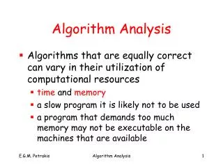
1. Algorithm Analysis • Algorithms that are equally correct can vary in their utilization of computational resources • time and memory • a slow program it is likely not to be used • a program that demands too much memory may not be executable on the machines that are available Algorithm Analysis

2. Memory - Time • It is important to be able to predict how an algorithm behaves under a range of possible conditions • usually different inputs • The emphasis is on the time rather than on the space efficiency • memory is cheap! Algorithm Analysis

3. Running Time • The time to solve a problem increases with the size of the input • measure the rate at which the time increases • e.g., linearly, quadratically, exponentially • This measure focuses on intrinsic characteristics of the algorithm rather than incidental factors • e.g., computer speed, coding tricks, optimizations, quality of compiler Algorithm Analysis

4. Additional Consideration • Sometimes, simple but less efficient algorithms are preferred over more efficient ones • the more efficient algorithms are not always easy to implement • the program is to be changed soon • time may not be critical • the program will run only few times (e.g., once a year) • the size of the input is always very small Algorithm Analysis

5. Bubble sort • Count the number of steps executed by the algorithm • step: basic operation • ignore operations that are executed a constant number of times for (i = 1; i < ( n – 1); i ++) for (j = n; j < (i + 1); j --) if ( A[ j – 1 ] > A[ j ] ) T(n) = c n2 swap(A[ j ] , A[ j – 1 ]); //step Algorithm Analysis

6. Asymptotic Algorithm Analysis • Measures the efficiency of a program as the size of the input becomes large • focuses on “growth rate”: the rate at which the running time of an algorithm grows as the size of the input becomes “big” • Complexity => Growth rate • focuses on the upper and lower bounds of the growth rates • ignores all constant factors Algorithm Analysis

7. Growth Rate • Depending on the order of n an algorithm can beof • Linear time Complexity: T(n) = c n • Quadratic Complexity: T(n) = c n2 • Exponential Complexity: T(n) = c nk • The difference between an algorithm whose running time is T(n) = 10n and another with running time is T(n) = 2n2 is tremendous • for n > 5 the linear algorithm is must faster despite the fact that it has larger constant • it is slower only for small n but, for such n, both algorithms are very fast Algorithm Analysis

8. Algorithm Analysis

9. Upper – Lower Bounds • Several terms are used to describe the running time of an algorithm: • The upper bound to its growth rate which is expressed by the Big-Oh notation • f(n) is upper bound of T(n)T(n) is in O(f(n)) • The lower bound to it growth rate which is expressed by the Omega notation • g(n) is lower bound of T(n)T(n) is in Ω(g(n)) • If the upper and lower bounds are the same T(n) is in Θ(g(n)) Algorithm Analysis

10. Big O (upper bound) • Definition: • Example: Algorithm Analysis

11. Properties of O • O is transitive: if • If • If • If Algorithm Analysis

12. More on Upper Bounds • T(n)  O(g(n))g(n) :upper boundfor T(n) • There exist many upper bounds • e.g., T(n) = n2O(n2) , O(n3)…O(n100) ... • Find the smallest upper bound!! • O notation “hides” the constants • e.g., cn2 , c2n2 , c!n2 ,…ckn2 O(n2) Algorithm Analysis

13. O in Practice • Among different algorithms solving the same problem, prefer the algorithm with the smaller “rate of growth” O • it will be faster for large n • Ο(1)< Ο(log n) < Ο(n)< Ο(n log n)< Ο(n2) < Ο(n3)< …< Ο(2n)< O(nn) • Ο(n), Ο(n log n), Ο(n2) < Ο(n3): polynomial • Ο(log n): logarithmic • O(nk), O(2n), (n!), O(nn): exponential!! Algorithm Analysis

14. n 100 20 200 500 1000 10-6 sec/command Complexity 1000n .02 .5 .1 .2 .5 1.0 1000nlogn .9 .3 .6 1.5 4.5 10 .04 .25 1.0 4.0 25 2min .08 1.0 10 1.0min 21min 27hrs .4 1.1 220day 125cent .0001 0.1 2.7hrs 1.0 35yrs 58min 50 Algorithm Analysis

15. Omega Ω (lower bound) • Definition: • g(n) is a lower bound of the rate of growth of f(n) • f(n) increases faster than g(n) as n increases • e.g: T(n) = 6n2 – 2n + 7 =>T(n) in Ω(n2) Algorithm Analysis

16. More on Lower Bounds • Ωprovides lower bound of the growth rate of T(n) • if there exist many lower bounds • T(n) = n4Ω(n), Ω(n2) ,  Ω(n3),  Ω(n4) • find the larger one=> T(n)  Ω(n4) Algorithm Analysis

17. ThetαΘ • If the lower and upper bounds are the same: • e.g.:T(n) = n3 +135n Θ(n3) Algorithm Analysis

18. Theorem: T(n)=Σ αi ni Θ(nm) • T(n)= αnnm +αn-1nm-1+…+α1n+ α0 O(nm) Proof: T(n)  |T(n)|  |αnnm|+|αm-1nm-1|+…|α1n|+|α0|  nm{|αm| + 1/n|αm-1|+…+1/nm-1|α1|+1/nm|α0|}   nm{|αm|+|αm-1|+…+|α1|+|α0|}  T(n)  O(nm) Algorithm Analysis

19. Theorem (cont.) • T(n) = αmnm + αm-1nm-1 +… α1n + α0 >= cnm + cnm-1 + … cn + c >= cnm where c = min{αm, αm-1,… α1,α0}=> T(n)Ω(nm) (a), (b) => Τ(n)  Θ(nm) Algorithm Analysis

20. Theorem: (a) (b) (either or ) Algorithm Analysis

21. Recursive Relations (1) Algorithm Analysis

22. Fibonacci Relation Algorithm Analysis

23. Fibonacci relation (cont.) • From (a), (b): • It can be proven that F(n)Θ(φn) where golden ratio Algorithm Analysis

24. Binary Search int BSearch(int table[a..b], key, n) { if (a > b) return (– 1) ; int middle = (a + b)/2 ; if (T[middle] == key) return (middle); else if ( key < T[middle] ) return BSearch(T[a..middle – 1], key); else return BSearch(T[middle + 1..b], key); } Algorithm Analysis

25. Analysis of Binary Search • Let n = b – a + 1: size of array and n = 2k – 1 for some k (e.g., 1, 3, 5 etc) • The size of each sub-array is 2k-1 –1 • c: execution time of first command • d: execution time outside recursion • T: execution time Algorithm Analysis

26. Binary Search (cont.) Algorithm Analysis

27. Binary Search for Random n • T(n) <= T(n+1) <= ...T(u(n)) where u(n)=2k – 1 • For some k: n < u(n) < 2n • Then, T(n) <= T(u(n)) = d log(u(n) + 1) + c => d log(2n + 1) + c =>T(n)  O(log n) Algorithm Analysis

28. Merge sort list mergesort(list L, int n) { if (n == 1) return (L); L1 = lower half of L; L2 = upper half of L; return merge (mergesort(L1,n/2), mergesort(L2,n/2) ); } n: size of array L (assume L some power of 2) merge: merges the sorted L1, L2 in a sorted array Algorithm Analysis

29. Algorithm Analysis

30. [25] [57] [48] [37] [12] [92] [86] [33] [25 57] [37 48] [12 92] [33 86] [25 37 48 57] [12 33 86 92] [12 25 33 37 48 57 86 92] Analysis of Merge sort log2n merges n steps per merge, log2n steps/merge => O(n log2n) Algorithm Analysis

31. Analysis of Merge sort • Two ways: • recursion analysis • induction Algorithm Analysis

32. Induction • Let T(n) = O(n log n) then T(n) can be written as T(n) <= a n log n + b, a, b > 0 • Proof: (1) for n = 1, true if b >= c1 (2) let T(k) = a k log k + b for k=1,2,..n-1 (3) for k=n prove that T(n) <= a nlog n+b For k = n/2 : T(n/2) <= a n/2 log n/2 + b therefore, T(n) can be written as T(n) = 2 {a n/2 log n/2 + b} + c2 n = a n(log n – 1)+ 2b + c2 n = Algorithm Analysis

33. Induction (cont.) • T(n) = a n log n – a n + 2 b + c2 n • Let b = c1 and a = c1 + c2=> T(n) <= (c1 + c2) n log n + c1=> T(n) <= C n log n + B Algorithm Analysis

34. Recursion analysis of mergesort • T(n) = 2T(n/2) + c2 n <= <= 4T(n/4) + 2 c2 n <= <= 8T(n/8) + 3 c2 n <= …… • T(n) <= 2i T(n/2i) + ic2n where n = 2i • T(n) <= n T(1) + c2 n log n =>T(n) < = n c1 + c2 n log n => T(n) <= (c1 + c2) n log n => T(n) <= C n log n Algorithm Analysis

35. Best, Worst, Average Cases • For some algorithms, different inputs require different amounts of time • e.g., sequential search in an array of size n • worst-case: element not in array => T(n) = n • best-case: element is first in array =>T(n) = 1 • average-case: element between 1, n =>T(n) = n/2 comparisons n Algorithm Analysis

36. Comparison • The best-case is not representative • happens only rarely • useful when it has high probability • The worst-case is very useful: • the algorithm performs at least that well • very important for real-time applications • The average-case represents the typical behavior of the algorithm • not always possible • knowledge about data distribution is necessary Algorithm Analysis