Download
1 / 43
430 likes | 517 Views
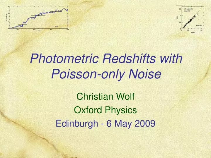
Photometric Redshifts with Poisson-only Noise. Christian Wolf Oxford Physics Edinburgh - 6 May 2009. Talk Outline. Why Photo-z’s? State of the Art Future challenges The 2 -empirical approach Persistent photo-z issues 2 -test: noisy model The PHAISE proposal.

E N D
Photometric Redshifts with Poisson-only Noise Christian Wolf Oxford Physics Edinburgh - 6 May 2009
Talk Outline • Why Photo-z’s? • State of the Art • Future challenges • The 2-empirical approach • Persistent photo-z issues • 2-test: noisy model • The PHAISE proposal
z < 0.01Stebbins & Whitford, AJ, 1948 I. Why Photo-z’s? Photography is deeper than spectroscopy! Baum 1957
Koo 1985 z/(1+z) ~ 0.04 @ z < 0.6 UBVI photographic plates Loh & Spillar 1986 Degrading all filter images to worst seeing important Star and galaxy library 10% outliers Half zphot wrong Insufficiently blue templates Photometric blends Half zspec wrong Blends Single-line detections Connolly et al. 1995 4-D space (z,U-B,B-R,R-I) Distribution has Df = 1.8 Colour ‘plane’ at z = [0,0.4] rotation after one filter Step-wise quadratic fits z/(1+z) < 0.04 @ z < 0.8 Photo-Zeeing in the 80’s/90’s
flux / qef 1000 nm 400 nm Redshift Errors & Resolution • Objects at different redshifts • Filterset 's fixed z = 0.843 G2 star vs.QSO z=3 z = 1.958 z = 2.828
rms 0.008 (R<21) 1 outlier rms 0.008 7%-20%outliers R=21.5 R=22.9 R=23.8 Galaxies at z~0.45 R=20 R=22 R=23.7 QSOsat z~2.8 II. State of the Art: Medium-band SEDs
ANN 2 template Collister & Lahav 2004 ~0% outliersz/(1+z)>0.1 rmsz/(1+z) = 0.023 Bias ~0.00 ~4%outliersz/(1+z)>0.1 rmsz/(1+z) = 0.042 Bias -0.017 State of the Art: ugriz-only ANN easy at z<1: no ambiguities… but wait for future data!
Catastrophic failures & misclassifications Large z errors Mean z bias Unrealistic z errors III. Future Challenges
Catastrophic failures & misclassifications Large z errors Mean z bias Unrealistic z errors Model ambiguities in colour space PDF too unconstrained PDF wrong Mismatch between data and model Origin of Challenges
Catastrophic failures & misclassifications Large z errors Mean z bias Unrealistic z errors Model ambiguities in colour space PDF too unconstrained PDF wrong Mismatch between data and model Use template error function Add more data Repair models Add priors Common Fixes
Super-large photo-z surveys for cosmology Now: PanStarrs, DES 2015++: LSST, IDEM Redshift bias from Model:data calibration Catastrophic outliers |z| ≈ |zoutlier| outlier Kitching, Taylor & Heavens: w ≈ 5z (3D cosmic shear) z = 0.01 unacceptable 1% outliers unacceptable Even spectroscopic surveys May have 1% wrong z’s Have incompleteness, i.e. more undiscovered outliers Why do These Matter?
data model Farb-bibliothek estimator Schätzer/Klassifikator result Back to The Principles: Overview empirical data or external template 2-fitting artificial neural netlearning algorithms spectral energydistribution PDF: p(z)
data model Farb-bibliothek estimator Schätzer/Klassifikator Frequentist precision statistics:= “Using what IS there: N(z)!” result Bayesian frontier exploration:= “What do we (not) know: p(z)=?” Back to The Principles: Overview empirical data or external template 2-fitting artificial neural netlearning algorithms spectral energydistribution PDF: p(z)
Model-Estimator Combinations • 2 • PDF Ambiguity warning • NN • No PDF, no warning • Template model • Can be extrapolated in z,mag • Calibration issues • Priors’ issues • Empirical model • Good priors • No calibration issues • Can not be extrapolated Code 2 NN Model Template Empirical
Model-Estimator Combinations • 2 • PDF Ambiguity warning • NN • No PDF, no warning • Template model • Can be extrapolated in z,mag • Calibration issues • Priors’ issues • Empirical model • Good priors • No calibration issues • Can not be extrapolated Code 2 NN Model Template Empirical ?
VI. The 2-empirical Approach • Goal • Combine 2-PDF with reliability of empirical model • Suggest • Replace templates with empirical model: has correct calibration & priors, but has also noise • However • PDF from 2-model testing only correct, if model correct and noise-free • Templates are noise-free but incorrect, so produce wrong PDF as well
From global fits (1980s) to local fits (2000s) Locally optimal solution Requires more data and computing power Kernel function Smooth over wide range for robust solution Smooth over small range for good representation Identical to 2-fitting if Model noise-free Gaussian kernel function with = data Colour given: Locally fitz(colour) z Compare: Kernel Regression
p z Equations: 2-testing • Probability of single given model object to produce data object • Parameter estimate • Expected error • Bimodality detection
Richards et al. 2007 For Now: Ignore Model Errors • SDSS QSO sample • Plenty of z-ambiguities • DR5: 75,770 objects split half:half into model:data • Pretend noise-free model
Fraction of outliers with|z| > 3z,limit (non-outliers) Photo-z “bias”= mean z of non-outliers Fraction of sample withz < z,limit Result: Non-bimodal Objects
Fraction of outliers with|z| > 3z,limit (non-outliers) z rms z Photo-z “bias”= mean z of non-outliers Fraction of sample withz < z,limit Results: Non-bimodal Objects
Result: Bimodal Objects • 15474 detected ambiguities • Two z’s given one colour • Need more data to break • Meanwhile • Trust more probable z • Mean p-ratio 78:22 predicts12077 right : 3397 wrong • 12051 right indeed! • Use two weighted results • Reliable: phigh ≈ fhigh • Sensitivity limits?8% 1:>20 and 1% 1:>50 • Undetected ambiguities inevitable (= erroneously uni-modal) • 30% of space, undetected 1:50-ambiguity 0.6% outliers
Histogram of zphot-estimatescount bimodal objects twiceusing p-weights Co-addition of all p(z)p(z) inform beyond zphot Result: Redshift Distributions
V. Persistent Photo-Z Issues • RMS redshift error • Has a floor supported by intrinsic scatter, deeper photometry useless • Redshift bias • Sub-samples can show local bias even when method globally bias-free • Catastrophic outliers • Faint ambiguities (extreme p-ratio) undetectable, only guard is all-out spectroscopy
Locally linear Error Floor from Intrinsic Scatter • Example: • QSO near (g-r)~1 or z~3.7 • z signal: Ly forest in g-band • Training sample in box • Redshift distribution:mean 3.66, rms 0.115 • RMS/(1+z) = 0.024 • Testing sample in box • RMS/(1+z) error 0.023
Not an issue whenplotted over zphot(by design!) Local Redshift Biases
Outliers from Undetected Ambiguities Model objects within kernel: Nprimary + N2nd = Nmodel,local Assume 2nd > 0; observe N2nd = 0: N2nd = 1 Hence, individual residual outlier risk: p2nd = 1/Nmodel,local
Incomplete targeting No problem, use weights Incomplete z recovery Model completeness f(z) Main reason: z different Missed “model outliers” Part of data PDF missing Maximum bias risk for objects at fixed colour Incomplete Models Mean Outliers
Incomplete targeting No problem, use weights Incomplete z recovery Model completeness f(z) Main reason: z different Missed “model outliers” Part of data PDF missing Maximum bias risk for objects at fixed colour Assume deep survey non-recov=0.2 |zout|=1 |z|=0.2 !!! Incomplete Models Mean Outliers Spectroscopic incompleteness deserves by far the greatest concern in empirical redshift estimation.* * |z|<10-3 means 99.9% completeness & reliability
q2 Model q1 q2 q1 2-Test: Noise-free Model p(data|model) = modelG2 (data) Gdata = G2 data = 2
q2 Model q1 q2 q2 q2 q1 q1 q1 Model VI. 2-Test: Noisy Model p(data|model) = modelG2 (data) Gdata = G2 data = 2 Gdata = GmodelG2 data = model + 2 2 = data - model
Data Noise vs. Model Noise • If data > model • Replace model point by Gaussian2 = data - model • If data ≈ model • When 2 0 then also Nmodel,local 0 and outlier risk 1 • Define p(z) only for regions larger than one object or… • If data < model • Larger target smoothing i.e. • Resample data point with resample = target - data • Replace model point by Gaussian 2 = target - model
Locally linear Model has scatterData has scatter At fixed colour: zphot = z True z scatter: Estimated photo-z error: Only equal if Error Propagation: Equations
Reconstruction of n(z) with Poisson precision Noisy Model, Noisy Data: n(z)=? Use noise levels of data = 0.1414model = 0.1000
Revisiting The data~model Case z rms z 2 0
Merge two approaches Model smoothing by kernel function Correct 2 error scale Strictly require Target smoothing scale constant across space Data error > model error Either from the start Or noise be introduced into data on purpose Desire for Better model photometry Constant data error scale Bright objects: errors in magnitudes Faint objects: errors in flux units (background) Or transform mag scale so that error constant Issues Varying exposure depth or interstellar extinction Unifying 2-testing with Kernel Regression - Practical Requirements
VII. The PHAISE Proposal PHoto-z Archive for Imaging Survey Exploitation • Gaussian-precision photo-z code & residual risk quantification from model incompleteness/size moves all attention to model • Residual outlier risk incomplete • Noise floor on n(z) 2n(z) 1/Nmodel,z-bin • The plan: A central repository for empirical model data • Avoid duplication of efforts, provide “the best empirical model” • Best-possible n(z)/photo-z quality from here, by definition • Dynamic and growing with time, well-known incompleteness • Web submission of small “photo-zeeing” jobs or customer installation for large applications (PanStarrs, LSST, …)
Calibrating new photo-z survey to PHAISE? Pure calculation of colour transformations reliable? Must observe calibration fields? Digesting diverse input Start with SDSS, VVDS, GOODS etc. Keeping track of sources of incompleteness 5-year goal: It works! Existing spectroscopic sources digested Incompleteness at R>22 too high for cosmology 10-year goal Deep complete spec-z survey fills gaps VIMOS, FMOS, SIDE,… “Fundamental” limits, e.g. source blending, AGN ... PHAISE Issues & Plan
Summary • Presented method delivers n(z|c) or photo-z with Poisson precision if model complete • Completeness of empirical spectroscopic model in faint regime is primary quality limit • Need deep, large, very complete spec survey! • Combine resources, do it once, and ABAP • Set up PHAISE, codes, technicalities • Propose “The Deep Complete” survey • Campaign for suitable optical + NIR instrumentation