Download
1 / 39
480 likes | 879 Views
IAU Comm.30, IAU XXVIII GA Beijing, August 2012. KVA. GRAVITATIONAL REDSHIFTS versus convective blueshifts , and wavelength variations across stellar disks Dainis Dravins – Lund Observatory , Sweden www.astro.lu.se /~ dainis. 100 years ago… . Predicted effects by gravity on light.

E N D
IAU Comm.30, IAU XXVIII GA Beijing, August 2012 KVA GRAVITATIONAL REDSHIFTS versus convective blueshifts, and wavelength variations across stellar disks Dainis Dravins – Lund Observatory, Sweden www.astro.lu.se/~dainis
Predicted effects by gravity on light A.Einstein, Annalen der Physik340, 848 (1911)
Freundlich’s attempts to verify relativity theory (I) Erwin Finlay Freundlich (1885-1964) worked to experimentally verify the predictions from Einstein’s theory of relativity and the effects of gravity on light. Klaus Hentschel: Erwin Finlay Freundlich and Testing Einstein’s Theory of Relativity, Archive for History of Exact Sciences 47, 243 (1994)
Freundlich’s attempts to verify relativity theory (II) Einsteinturm, Potsdam-Telegrafenberg Klaus Hentschel: Erwin Finlay Freundlich and Testing Einstein’s Theory of Relativity, Archive for History of Exact Sciences 47, 243 (1994)
Expected gravitational redshifts D. Dravins IAU Symp. 210
Expected gravitational redshifts R.F.Griffin: Spectroscopic Binaries near the North Galactic Pole. Paper 6: BD 33° 2206, J.Astrophys.Astron. 3, 383 (1982)
Astrometric radial velocities Dravins, Lindegren & Madsen, A&A 348, 1040
Pleiades from Hipparcos Proper motions over 120,000 years
Apparent radial velocity vs. rotation? S.Madsen, D.Dravins, H.-G.Ludwig, L.Lindegren: Intrinsic spectral blueshifts in rapidly rotating stars?, A&A 411, 581
Differential velocities within open clusters
Different “velocities” ─ giants vs. dwarfs? B.Nordström, J.Andersen, M.I.Andersen: Critical tests of stellar evolution in open clusters II. Membership, duplicity, and stellar and dynamical evolution in NGC 3680, Astron. Astrophys. 322, 460
M67 Dean Jacobsen, astrophoto.net
Searching for gravitational redshifts in M67 Dean Jacobsen, astrophoto.net M67 color–magnitude diagram with well-developed giant branch. Filled squares denote single stars. M67 (NGC 2682) open cluster in Cancer contains some 500 stars; age about 2.6 Gy, distance 850 pc. L.Pasquini, C.Melo, C.Chavero, D.Dravins, H.-G.Ludwig, P.Bonifacio, R.DeLa Reza: Gravitational redshifts in main-sequence and giant stars, A&A 526, A127 (2011)
Searching for gravitational redshifts in M67 Radial velocities in M67: No difference seen between giants (red) and dwarfs (dashed) Radial velocities in M67 with a superposed Gaussian centered on Vr= 33.73, σ = 0.83 km s−1 L.Pasquini, C.Melo, C.Chavero, D.Dravins, H.-G.Ludwig, P.Bonifacio, R.DeLa Reza: Gravitational redshifts in main-sequence and giant stars, A&A 526, A127 (2011)
AN ”IDEAL” STAR? Solar disk June 12, 2009 GONG/Teide
Solar Optical Telescope on board HINODE (Solar-B) G-band (430nm) & Ca II H (397nm) movies
Spectral scan across the solar surface. Left: H-alpha line Right: Slit-jaw image Big Bear Solar Observatory
“Wiggly” spectral lines of stellar granulation (modeled) Disk-center Fe I profiles from 3-D hydrodynamic model of the metal-poor star HD 140283 in NLTE and LTE. Top: Synthetic “wiggly-line” spectra across stellar surface. Curves show equivalent widths W along the slit. Bottom: Spatially resolved profiles; average is red-dotted. N.G.Shchukina, J.TrujilloBueno, M.Asplund, Astrophys.J.618, 939 (2005)
SPECTRAL LINES FROM 3-D HYDRODYNAMIC SIMULATIONS Spatially averaged line profiles from 20 timesteps, and temporal averages. = 620 nm = 3 eV 5 line strengths GIANT STAR Teff= 5000 K log g [cgs] = 2.5 (approx. K0 III) (Models by Hans-Günter Ludwig, LandessternwarteHeidelberg)
SPECTRAL LINES FROM 3-D HYDRODYNAMIC SIMULATIONS Spatially and temporally averaged line profiles. = 620 nm = 1, 3, 5 eV 5 line strengths GIANT STAR Teff= 5000 K log g [cgs] = 2.5 (approx. K0 III) Stellar disk center; µ = cos = 1.0 (Models by Hans-Günter Ludwig, LandessternwarteHeidelberg)
SPECTRAL LINES FROM 3-D HYDRODYNAMIC SIMULATIONS Spatially and temporally averaged line profiles. = 620 nm = 1, 3, 5 eV 5 line strengths GIANT STAR Teff= 5000 K log g [cgs] = 2.5 (approx. K0 III) Off stellar disk center; µ = cos = 0.59 (Models by Hans-Günter Ludwig, LandessternwarteHeidelberg)
SPECTRAL LINES FROM 3-D HYDRODYNAMIC SIMULATIONS Spatially and temporally averaged line profiles. = 620 nm = 1, 3, 5 eV 5 line strengths SOLAR MODEL Teff= 5700 K log g [cgs] = 4.4 (G2 V) Solar disk center; µ = cos = 1.0 (Models by Hans-Günter Ludwig, LandessternwarteHeidelberg)
SPECTRAL LINES FROM 3-D HYDRODYNAMIC SIMULATIONS Spatially and temporally averaged line profiles. = 620 nm = 1, 3, 5 eV 5 line strengths SOLAR MODEL Teff= 5700 K log g [cgs] = 4.4 (G2 V) Off solar disk center; µ = cos = 0.59 (Models by Hans-Günter Ludwig, LandessternwarteHeidelberg)
Cool-star granulation causes convective lineshifts on order 300 m/s
Bisectors of the same spectral line in different stars Adapted from Dravins & Nordlund, A&A 228, 203 From left: Procyon (F5 IV-V), Beta Hyi (G2 IV), Alpha Cen A (G2 V), Alpha Cen B (K1 V). In stars with “corrugated” surfaces, convective blueshifts increase towards the stellar limb G2 IV G2 V F5 K1 Velocity [m/s]
Searching for gravitational redshifts in M67 Calculated convective wavelength shifts for Fe I lines in dwarf (red crosses) and giant models (squares). Gravitational redshift predictions vs. mass/radius ratio (M/R) (dashed red) do not agree with observations. L.Pasquini, C.Melo, C.Chavero, D.Dravins, H.-G.Ludwig, P.Bonifacio, R.DeLa Reza: Gravitational redshifts in main-sequence and giant stars, A&A 526, A127 (2011)
Variable gravitational redshift in variable stars? H.M.Cegla, C.A.Watson,T.R.Marsh, S.Shelyag, V.Moulds, S.Littlefair, M.Mathioudakis, D.Pollacco, X.Bonfils Stellar jitter from variable gravitational redshift: Implications for radial velocity confirmation of habitable exoplanets MNRAS 421, L54 (2012) Stellar radius changes required to induce a δVgrav equivalent to an Earth-twin RV signal. Circles represent (right to left) spectral types: F0, F5, G0, G2, G5, K0, K5 and M0. Dashed curves represent stellar radius variations of 50, 100 and 300 km
Exoplanet transit Selecting a small portion of the stellar disk (Hiva Pazira, Lund Observatory)
Spatially resolved stellar spectroscopy Left: Integratedlineprofiles Vrot = 2, 40, 120 km/s Right: Line behind planet Top: Noise-free Bottom: S/N = 300, R=300,000 (HivaPazira, Lund Observatory)
Spatially resolved stellar spectroscopy Synthetic line profiles across stellar disks Examples of synthetic line profiles from hydrodynamic 3-D stellar atmospheres. Curves are profiles for different positions on the stellar disk, at some instant in time. Black curves are at disk-center; lower intensities of other curves reflect the limb darkening. Top: Solar model; Fe I, 620 nm, 1 eV. Bottom: Giant model; Fe I, 620 nm, 3eV. Disk locations cos = µ = 1, 0.87, 0.59, 0.21. Simulation by Hans-Günter Ludwig (LandessternwarteHeidelberg)
Spatially resolved spectroscopy with ELTs Left: Hydrodynamic simulation of the supergiant Betelgeuse (B.Freytag) Right: Betelgeuse imaged with ESO’s 8.2 m VLT (Kervella et al., A&A, 504, 115) Top right: 40-m E-ELT diffraction limits at 550 nm & 1.04 μm.. HivaPazira(Lund Observatory)