Download

1 / 14
140 likes | 281 Views
High Accuracy Schemes for Inviscid Traffic Models. Eric Liu 18.336 Final Project. The Payne-Whitham Model. Models the density and velocity of cars Conservation of cars

E N D
High Accuracy Schemesfor Inviscid Traffic Models Eric Liu 18.336 Final Project
The Payne-Whitham Model • Models the density and velocity of cars • Conservation of cars • Drivers change their speed with finite acceleration: 1) according to traffic conditions ahead, 2) to maintain a steady velocity (e.g. speed limit) • No movement at road’s max density
Numerical Approach: Overview • Roe’s Approximate Flux Solver • Monotone Upstream-centered Schemes for Conservation Laws (MUSCL) • Linear (2nd order) spatial discretization • Quadratic (3rd order) • Flux-Limiters • van Leer, superbee, minmod, van Albada • Time-Stepping • RK4 (standard method) • SSP-RK3 (Strong Stability Preserving)
Linear MUSCL • Uses linear reconstruction inside each cell • Result uses the difference between successive cell averages and the ratio of successive slopes:
Linear MUSCL • Resulting semi-discretization: • Better resolution of sharp (shock) features than diffusive first order schemes • 2nd order accurate in space (smooth solution) • Not TVD: requires flux-limiters to avoid spurious oscillations around shocks
SSP-RK3 • Advantage of SSP methods: • Guarantees that time-step restrictions will be no worse than with Forward Euler • Holds all oscillation diminishing properties of Forward Euler + TVD schemes • Downsides: • Formulations do not exist for arbitrarily high orders of convergence • Methods beyond 3rd order are expensive
Convergence Rates • No source term • Similar to the Shallow Water Equations, except with a logarithmic pressure (instead of linear) • Source term
Ripples? • Despite the use of TVD spatial discretizations and SSP time stepping, ripples (high frequency oscillations) were sometimes observed. • Only occurs under 1) backward traveling shocks • Observed for higher order AND first order schemes! • Ripple train width decreases with: • increasing grid resolution • increasing solution order • Ripple train maximum amplitude does not decrease significantly with more resolution
Conclusion: Methods • Higher order schemes work well on the Payne-Whitham model • TVD algorithms in space • SSP time stepping • Linear reconstruction leads to sharper shock resolution than quadratic methods (tend to be more dispersive) • Tend to overshoot more than quadratic methods at lower grid resolution • Quadratic performance likely limited by inadequate limiters • Recent limiters by Colella have improved performance; these were not implemented.
Conclusion: Ripples • Very surprising observation • Analytic results by Flynn et al. imply that the ripples are numerical artifacts • Exact solution may be unstable, so disturbances associated with floating point arithmetic induce the ripples • Ripple train width may decrease with increasing resolution due to better resolution of the ripples (i.e. less downstream pollution) • Is consistent with the ripples’ non-diminishing amplitude
Roe’s Approximate Flux • Solving a nonlinear Riemann problem is generally hard • Interpolates the flux Jacobian linearly between the left/right interface states • Selects average flux Jacobian by “Roe-Averaging” the left/right states. • Exact solution if the interfacial jump is a single discontinuous wave
Roe’s Approximate Flux • Roe (rho?)-Average: • Computing the Roe Flux: • Uses F (physical flux) and , the flux Jacobian