Download
1 / 104
1.04k likes | 1.24k Views
The Batik Trick a Physically Plausible Simulation of Traditional Batik Painting using Distance Transforms, Distance Transforms, and Distance Transforms by Brian Wyvill and Kees van Overveld. contents The Art of Batik Painting The Visual Effects and their Causes Distance Transforms

E N D
The Batik Trick a Physically Plausible Simulation of Traditional Batik Painting using Distance Transforms, Distance Transforms, and Distance Transforms by Brian Wyvill and Kees van Overveld
contents • The Art of Batik Painting • The Visual Effects and their Causes • Distance Transforms • A Batik Simulator • Results, Conclusions and Summary
1.The Art of Batik Painting • Batik (American: ba-teek’; Correct: bah’-tik) • origins unknown; 2000 years old; Middle-east, India or Central Asia? • most prevalent: Indonesian island of Java; since 14th or 15th century • http://www.story-of-batik.com/html/history_of_batik.html
1.The Art of Batik Painting the wax-gorithm: • while (not ready){ • dye entire cloth with color C; • for(p in uncovered region) p.color *= C; • wash off color on wax-covered areas (if any); • cover part of exposed region with wax; • if(expensive || just for fun) remove wax from some regions; • } • correct mistakes or add painted details; • sell; • // you should be rich now !!!
1.The Art of Batik Painting example
2.The Visual Effects and their Cause (the phenomenology of dye absorption and wax cracking)
2.The Visual Effects and their Cause (the phenomenology of dye absorption and wax cracking) non-homogenous cloth absorption rates:
2.The Visual Effects and their Cause (the phenomenology of dye absorption and wax cracking) non-homogenous cloth absorption rates: cracks occur in time-order instead of all-at-once so there are few crack crossings but most T-junctions ... because crack-propagation is a causal process: cracks run until they encounter another (earlier) crack or the bound of the wax
2.The Visual Effects and their Cause (the phenomenology of dye absorption and wax cracking) non-homogenous cloth absorption rates: cracks occur in time-order cracks often end in maximally concave regions of wax borders ..instead of... ...because it is energetically cheap to have shorter cracks
2.The Visual Effects and their Cause (the phenomenology of dye absorption and wax cracking) non-homogenous cloth absorption rates: cracks occur in time-order cracks often end in maximally concave regions of wax borders cracks erode, so older cracks result in wider dye traces than younger cracks
2.The Visual Effects and their Cause (the phenomenology of dye absorption and wax cracking) non-homogenous cloth absorption rates: cracks occur in time-order cracks often end in maximally concave regions of wax borders cracks erode, so older cracks result in wider dye traces than younger cracks junction regions are fragile, so wax breaks off, leaving widened ‘younger’ crack ends
2.The Visual Effects and their Cause (the phenomenology of dye absorption and wax cracking) non-homogenous cloth absorption rates cracks occur in time-order cracks often end in maximally concave regions of wax borders cracks erode, so older cracks result in wider dye traces than younger cracks junction regions are fragile, so wax breaks off, leaving widened ‘younger’ crack ends ...this will be achieved by an appropriate noise function
2.The Visual Effects and their Cause (the phenomenology of dye absorption and wax cracking) non-homogenous cloth absorption rates cracks occur in time-order cracks often end in maximally concave regions of wax borders cracks erode, so older cracks result in wider dye traces than younger cracks junction regions are fragile, so wax breaks off, leaving widened ‘younger’ crack ends ...whereas various Distance Transforms will be used for these
3.Distance Transforms (Jack-of-all-trades in image processing)
3.Distance Transforms (Jack-of-all-trades in image processing) • formal definition: • for a set S, and a metric | , |: S S • and a subset VS, we define • s, sS: D(s)=MIN(v:v V:|s-v|)
arb. shape V small D: V’s border small D: V’s border small D: V’s border large D: diamond large D: circle large D: square 3.Distance Transforms (examples) in geometry: for small distance D: for large distance D: L1 -metric L2 -metric L -metric
3.Distance Transforms (observations) • distance transform models decreasing influence at larger D: shape details are lost (Huygens’ principle) • shape of (D=const)-contour dominates for large D • distance transform is related to • Minkowsky sum • Voronoi diagram • low-pass filtering & multi-scale • implicit surfaces • Dijsktra’s shortest path (discrete S) • most preferred metric: L2 (independent of coordinate system) • brute force calculation requires O(|S||V|) calculations • approximations require O(n |S|) calculations
3.Distance Transforms (fast approximation) a two-pass algorithm for the Distance Transform: for(pixel p in V) D(p)=0; for(pixel p in S\V) D(p)=infinity; for(pixel p: scan from top left to bottom right){ for(pixel n in upper left half Neighborhood(p)) if(D(n)+|n-p|>D(p))D(p)=D(n)+|n-p|; } for(pixel p: scan from bottom right to top left){ for(pixel n in lower right half Neighborhood(p)) if(D(n)+|n-p|>D(p))D(p)=D(n)+|n-p|; } (optionally, smooth D(p) with a suitable relaxation)
3.Distance Transforms (fast approximation) 0 0 0 0 0
3.Distance Transforms (fast approximation) 0 0 0 0 0
3.Distance Transforms (fast approximation) 0 0 0 0 0
3.Distance Transforms (fast approximation) 0 1 0 0 0 0
3.Distance Transforms (fast approximation) 0 1 0 0 0 0
3.Distance Transforms (fast approximation) 0 1 1.41 0 0 0 0
3.Distance Transforms (fast approximation) 0 1 1.41 2.41 0 0 0 0
3.Distance Transforms (fast approximation) 0 1 1.41 2.41 3.41 0 0 0 0
3.Distance Transforms (fast approximation) 0 1 1.41 2.41 3.41 0 0 1 0 0
3.Distance Transforms (fast approximation) 0 1 1.41 2.41 3.41 0 0 1 1.41 0 0
3.Distance Transforms (fast approximation) 0 1 1.41 2.41 3.41 0 0 1 1.41 2.41 0 0
3.Distance Transforms (fast approximation) 0 1 1.41 2.41 3.41 this is wrong: it should be 2.82. Don’t panic, just wait and see 0 0 1 1.41 2.41 0 0
3.Distance Transforms (fast approximation) 0 1 1.41 2.41 3.41 0 0 1 1.41 2.41 0 0 1
3.Distance Transforms (fast approximation) 0 1 1.41 2.41 3.41 0 0 1 1.41 2.41 0 0 1 2
3.Distance Transforms (fast approximation) 0 1 1.41 2.41 3.41 0 0 1 1.41 2.41 0 0 1 2 1.41
3.Distance Transforms (fast approximation) 0 1 1.41 2.41 3.41 0 0 1 1.41 2.41 0 0 1 2 1.41 1
3.Distance Transforms (fast approximation) 0 1 1.41 2.41 3.41 0 0 1 1.41 2.41 0 0 1 2 1.41 1 1
3.Distance Transforms (fast approximation) 0 1 1.41 2.41 3.41 0 0 1 1.41 2.41 0 0 1 2 1.41 1 1 1.41
3.Distance Transforms (fast approximation) 0 1 1.41 2.41 3.41 0 0 1 1.41 2.41 0 0 1 2 1.41 1 1 1.41 2.41
3.Distance Transforms (fast approximation) 0 1 1.41 2.41 3.41 0 0 1 1.41 2.41 0 0 1 2 1.41 1 1 1.41 2.41 2.82
3.Distance Transforms (fast approximation) 0 1 1.41 2.41 3.41 0 0 1 1.41 2.41 0 0 1 2 1.41 1 1 1.41 2.41 2.82 2.41
3.Distance Transforms (fast approximation) 0 1 1.41 2.41 3.41 0 0 1 1.41 2.41 0 0 1 2 1.41 1 1 1.41 2.41 2.82 2.41 2
3.Distance Transforms (fast approximation) 0 1 1.41 2.41 3.41 0 0 1 1.41 2.41 0 0 1 2 1.41 1 1 1.41 2.41 2.82 2.41 2 2
3.Distance Transforms (fast approximation) 0 1 1.41 2.41 3.41 0 0 1 1.41 2.41 0 0 1 2 1.41 1 1 1.41 2.41 2.82 2.41 2 2 2.41
3.Distance Transforms (fast approximation) 0 1 1.41 2.41 3.41 0 0 1 1.41 2.41 0 0 1 2 1.41 1 1 1.41 2.41 2.82 2.41 2 2 2.41 2.82
3.Distance Transforms (fast approximation) 0 1 1.41 2.41 3.41 0 0 1 1.41 2.41 0 0 1 2 1.41 1 1 1.41 2.41 2.82 2.41 2 2 2.41 2.82 next we revert the scanning direction
3.Distance Transforms (fast approximation) 0 1 1.41 2.41 3.41 0 0 1 1.41 2.42 0 0 1 2 1.41 1 1 1.41 2.41 3.82 2.82 2.41 2 2 2.41 2.82
3.Distance Transforms (fast approximation) 0 1 1.41 2.41 3.41 0 0 1 1.41 2.41 0 0 1 2 2.41 1.41 1 1 1.41 2.41 3.82 2.82 2.41 2 2 2.41 2.82
3.Distance Transforms (fast approximation) 0 1 1.41 2.41 3.41 0 0 1 1.41 2.41 0 0 1 2 3.41 2.41 1.41 1 1 1.41 2.41 3.82 2.82 2.41 2 2 2.41 2.82
3.Distance Transforms (fast approximation) 0 1 1.41 2.41 3.41 0 0 1 1.41 2.41 1 0 0 1 2 3.41 2.41 1.41 1 1 1.41 2.41 3.82 2.82 2.41 2 2 2.41 2.82
3.Distance Transforms (fast approximation) 0 1 1.41 2.41 3.41 0 0 1 1.41 2.41 2 1 0 0 1 2 3.41 2.41 1.41 1 1 1.41 2.41 3.82 2.82 2.41 2 2 2.41 2.82