Download
1 / 35
360 likes | 527 Views
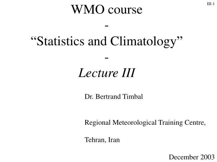
WMO course - “Statistics and Climatology” - Lecture III. Dr. Bertrand Timbal Regional Meteorological Training Centre, Tehran, Iran December 2003. Statistics and Climatology: Lecture III. Review some classical statistical tools.

E N D
WMO course-“Statistics and Climatology” - Lecture III Dr. Bertrand Timbal Regional Meteorological Training Centre, Tehran, Iran December 2003
Statistics and Climatology:Lecture III Review some classical statistical tools Statistics of the Climate system--- Spatio-temporal linkages within the system Overview: • Links within the system: the example of ENSO • Regression and correlation of variables • Spatial structures: reduction of the degree of freedom
El Niño / La Niña : a large scale feature Schematic of summer La Niña conditions across the Equatorial Pacific Ocean
El Niño / La Niña: a large scale feature Schematic of summer EL Niño conditions across the Equatorial Pacific Ocean
El Niño: a large scale feature Thermocline: Layer of strong temp gradient around 20C • Temperature, along an equatorial • longitude-depth section • Anomalies are relevant for interannual variability • Observed with the TAO: array of buoys in the Tropical Pacific • Thermocline movements important for seasonal forecasting
El Niño: sub-surface ocean anomalies • Anomalous warm water accumulated • at depth in the West Pacific and travel across the basin along the thermocline • The predictability comes from the slow moving ocean anomalies 97-98 El Niño formation
Transition to the 98-99 La Niña
El Niño: Global Tele-connections Courtesy of NOAA
La Niña: Global Tele-connections Courtesy of NOAA
El Niño: impact on Australian rainfall Stratification of the mean climate based on ENSO phases
La Niña: impact on Australian rainfall Stratification of the mean climate based on ENSO phases
El Niño: global impact on rainfall Probability of exceeding median rainfall for Cold, Neutral and Warm conditions in the Equatorial Pacific Ocean (Data for 1900-1997) Stratification of the mean climate based on ENSO phases.
El Niño: impact on Australian Wheat Yields
How to best express these relationships ? • Links within the climate system exist: • El Niño is a planetary scale phenomenon • Several variables exhibit coherent variations (correlation) • Distant teleconnections are observed (lag correlation) • Probabilities are shifted by ENSO phases (predictable)
Statistics of the Climate system--- Spatio-temporal linkages within the system Overview: • Links within the system: the example of ENSO • Regression and correlation of variables • Spatial structures: reduction of the degree of freedom
Simple model: Least-Squares Regression • Correlation: • Pearson ordinary correlation (r) • a is the intercept for X=0 • b is the slope: • r2 isthe amount of variance explained Regression:
Role of outliers: • Outlier detection method to find observations with large influence • Problem often arises from either erroneous data or small sample • Graphical visualisation is essential r = 0.457 r = 0.336 In this example, out of 100 points, only one data is different ! Courtesy of J. Stockburger
Graphical visualisation of correlation Perfect relationship affected by one data False correlation based on one erroneous data The relationship is not linear. In all cases, the correlation is r=0.816 but … Correlation is not robust and resistant …. Instead we can use the rank correlation: correlation based on ranked data
An example of a non linear relation Rainfall and river flow Annual SW WA Rainfall Annual SW WA Rainfall 950 950 750 750 550 550 350 350 1880 1900 1920 1940 1960 1980 2000 1880 1900 1920 1940 1960 1980 2000 AswWArain 20 per. Mov. Avg. (AswWArain) AswWArain 20 per. Mov. Avg. (AswWArain) Courtesy of S. Power
Correlation is not causation! Is ENSO forced by Australian rainfall? or Are Australian rainfall affected by ENSO? Correlations between seasonal rain and SOI • Correlation does not imply causation • Simultaneous evolution • Others techniques are needed: • Path analysis (Blalock, 1971) • Temporal precedence Courtesy of W. Drosdowsky
Lag Correlation and auto-correlation • Lag correlation of a series with itself is auto-correlation at lag-k: • Meteorological variables are auto-correlated (persistence) • Violate the independent data assumption effective sample size • Hypothesis testing • Variance estimate Lagged correlation between the SOI and cyclone formation • (Prior) Lag correlations exhibit the dependence between variables • Predictability arises from lag correlation
Correlation in the climate system: • Correlation coefficientes express the part of the variation of two variables which are linked (no causality) • Correlation assumes normality (!) and linear relation (!) • A more robust coefficient is the rank correlation • Lag correlation is useful for causality and predictability • Auto-correlation of meteorological data has serious consequences for the use of statistics in climate
Statistics of the Climate system--- Spatio-temporal linkages within the system Overview: • Links within the system: the example of ENSO • Regression and correlation of variables • Spatial structures: reduction of the degree of freedom
Spatial structure in climate data • Several motivations to identify large scale spatial features: • Data are not spatially independent: spatial correlation • Large scale structures are more coherent and predictable • Extract the large scale climate signal • Reduce the weather noise associated with small scales • Smaller degree of freedom and reduced data set • Identify useful relationships to exploit for climate forecasting
Principal-Component (EOF) Analysis • Objective: • To reduce the original data set to a new data set of (much) fewer variables • To condense a large fraction of the variance of the original dataset • To explore large multivariate data sets (spatial and temporal variation) • Calculation: • PCA are done on anomalies • Based on the covariance [S] or the • correlation [R] matrix of a vector X: XTX • The principal components are the • projection of X on the eigenvectors of [S]: ei • orthogonal one to an other: new coordinate system • maximise the variance: measured by the eigenvalues (λi)
Principal-Component (EOF) Analysis • Eigenvectors (PCA) are orthogonal • Strong constraint for small domain (Jolliffe, 1989) • Typically the 2nd PC is a dipole (not necessarily meaningful) • The number of PCs to be consider is based on the eigenvalues
EOFs of combined fields: Courtesy of M. Wheeler 200 hPa 850 hPa
The phase-space representation of the MJO M(t)= [RMM1(t),RMM2(t)] Vector M traces: - large anti-clockwise circles about the origin when the MJO is strong. - random jiggles around the origin when the MJO is weak. For compositing, we define the 8 equal-angle phases as labeled, and described by the angle Φ = tan-1[RMM2(t)/RMM1(t)] Courtesy of M. Wheeler Southern Summer = DJFMA
MJO propagation based on vector M in the two dimensional phase space OLR contour interval = 4 Wm-2 blue negative 850 hPa wind Max vector = 4.5 ms-1 Courtesy of M. Wheeler
Rotated PCs • Facilitate physical interpretation • Review by Richman (1986) and by Jolliffe (1989, 2002) • New set of variable: RPCs • Varimax is a very classic rotation technique (many others) First two rotated PCAs of Indian/Pacific SSTAs using data from Jan 1949 to Dec 1991. Courtesy of W. Drosdowsky
Other multivariate analyses • Extended EOFs and Complex (Hilbert) EOFs are two classical extensions of PCs • Canonical Correlation Analysis: extension of PCA to two multivariate data sets: forecasting one variable with the other (book by Wilks, 1995). • Principal Orthogonal Pattern (POP) and (PIP), SVD are other techniques used (book by von Storch and Navarra, 1995 and von Storch and Zwiers, 1999) • Discriminant analysis (e.g. the operational seasonal forecast of the BoM): the conditioning is on the predictand and in a sense the reverse conditional probabilities are estimated from the data, and Bayes theorem is used to invert these (article by Drosdowsky and Chambers, 2001) • Analogue (lecture 7), clustering (book by Wilks, 1995) and NHMM (next slide) are other techniques dealing with classification. • All techniques can be use for forecasting and downscaling
L 1012 3 .2 .4 .6 .8 1 1016 H H Type 1016 1012 1004 1000 1008 L 1012 5 .2 .4 .6 .8 1 1016 1020 Type 1016 H 1012 An other downscaling approach Non-homogeneous Hidden Markov Model: makes use of non observed “hidden” weather states which are related to observed rainfall structures Courtesy of S. Charles
Tool box to analyse our dynamic climate system …. and … basis for climate forecasting Summary: • Many interactions in the system correlation • Many issues with correlation: robustness, causality • Large scale structure exist multivariate analyses • Useful for filtering, organizing and reducing the noise in data • Forecasting uses many of these statistical tools