Overview of the Phase Problem

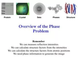
Protein Crystal Data Phases Structure Overview of the Phase Problem Remember We can measure reflection intensities We can calculate structure factors from the intensities We can calculate the structure factors from atomic positions We need phase information to generate the image

What is the Phase Problem X-ray Diffraction Experiment All phase information is lost x,y.z Fhkl [Real Space] [Reciprocal Space] In the X-ray diffraction experiment photons are reflected from the crystal lattice (planes) in different directions giving rise to the diffraction pattern. Using a variety of detectors (film, image plates, CCD area detectors) we can estimate intensities but we loose any information about the relative phase for different reflections.

Phases Let’s define a phase for an individual atom, fj An atom at xj=0.40, yj=0.25, zj=0.10 for plane [213] fj = 2p[ 2•(0.40) + 1•(0.25) + 3•(0.10)] = 2p(1.) For k = 0 (a 2D case) then For plane [201] fj = 2p[ 2•(0.40) + 1•(0.10)] = 2p(0.) Now to understand what this means….

0° 360° 0 c A A 2p 201 planes B B D D C C 720° 0.4, y, 0.1 E E H H 4p F F G G I I 1080° a 6p 201 Phases fD = 2p[ 2•(0.40) + 1•(0.10)] = 2p(0.)

In General for Any Atom (x, y, z) a dhkl 6π dhkl 4π Atom (j) at x,y,z dhkl 2π φ 0 c Plane hkl Remember: We express any position in the cell as (1) fractional coordinates pxyz = xja+yjb+zjc (2) the sum of integral multiples of the reciprocal axes hkl = ha* + kb* + lc*

Phase for Any Atom

Fourier transform Inverse Fourier transform Why Do We Need the Phase? Structure Factor Electron Density In order to reconstruct the molecular image (electron density) from its diffraction pattern both the intensity and phase, which can assume any value from 0 to 2, of each of the thousands of measured reflections must be known.

Importance of Phases Hauptman amplitudes with Hauptman phases Karle amplitudes with Karle phases Hauptman amplitudes with Karle phases Karle amplitudes with Hauptman phases Phases dominate the image! Phase estimates need to be accurate

The phase problem can be best understood from a simple mathematical construct. • The structure factors (Fhkl) are treated in diffraction theory as complex quantities, i.e., they consist of a real part (Ahkl) and an imaginary part (Bhkl). • If the phases, hkl, were available, the values of Ahkl and Bhkl could be calculated from very simple trigonometry: • Ahkl = |Fhkl| cos (hkl) • Bhkl= |Fhkl| sin (hkl) • this leads to the relationship: • (Ahkl)2 + (Bhkl)2 = |Fhkl|2 = Ihkl Understanding the Phase Problem

(Ahkl)2 + (Bhkl)2 = |Fhkl|2 = Ihkl Argand Diagram The above relationships are often illustrated using an Argand diagram (right). From the Argand diagram, it is obvious that Ahkl and Bhkl may be either positive or negative, depending on the value of the phase angle, hkl. Note: the units of Ahkl, Bhkl and Fhkl are in electrons.

The Structure Factor f0 sinΘ/λ Atomic scattering factors Here fj is the atomic scattering factor The scattering factorfor each atom type in the structure is evaluated at the correct sinΘ/λ. That value is the scattering ability of that atom. Remember We now have an atomic scattering vector with a magnitude f0 and direction φj .

The Structure FactorSum of all individual atom contributions imaginary Resultant Fhkl Individual atom fjs Bhkl real Ahkl

Remember the electron density (image of the molecule) is the Fourier transform of the structure factor Fhkl. Thus Electron Density Here V is the volume of the unit cell In practice, the electron density for one three-dimensional unit cell is calculated by starting at x, y, z = 0, 0, 0 and stepping incrementally along each axis, summing the terms as shown in the equation above for all hkl (as limited by the resolution of the data) at each point in space.

Solving the Phase Problem Small molecules Direct Methods Patterson Methods Molecular Replacement Macromolecules Multiple Isomorphous Replacement (MIR) Multi Wavelength Anomalous Dispersion (MAD) Single Isomorphous Replacement (SIR) Single Wavelength Anomalous Scattering (SAS) Molecular Replacement Direct Methods (special cases)

Solving the Phase Problem SMALL MOLECULES The use of Direct Methods has essentially solved the phase problem for well diffracting small molecule crystals. MACROMOLECULES Today, anomalous scattering techniques such as MAD or SAS are the most common techniques used for de novo structure determination of macromolecules. Both techniques require the presence of one or more anomalous scatterers in the crystal.

SIR and SAS Methods • Need a heavy atom (lots of electrons) or a anomalous scatterer (large anomalous scattering signal) in the crystal. • SIR - heavy atoms usually soaked in. • SAS - anomalous scatterers usually engineered in as selenomethional labels. Can also be soaked. • SIR collect a native and a derivative data set (2 sets total). SAS collect one highly redundant data set and keep anomalous pairs separate during processing. • SAS - may want to choose a scatterer or wavelength that enhances the anomalous signal. • Must find the heavy atoms or anomalous scatterers • can use Patterson analysis or direct methods. • Must resolve the bimodal ambiguity. • use solvent flattening or similar technique

Heavy Atom Derivatives Heavy atom derivatives MUST be isomorphous Heavy atom derivatives are generally prepared by soaking crystals in dilute (2 - 20 mM) solutions of heavy atom salts (see Table II below for some examples). Crystal cracking is generally a good indication that that heavy atom is interacting with the crystal lattice, and suggests that a good derivative can be obtained by soaking the crystal in a more dilute solution. Once derivative data has been collected, the merging R factor (Rmerge) between the native and derivative data sets can be used to check for heavy atom incorporation and isomorphism. Rmerge values for isomorphous derivatives range from 0.05 to 0.15. Values below 0.05 indicate that there is little heavy atom incorporation. Values above 0.15 indicate a lack of isomorphism between the two crystals.

Finding the Heavy Atoms or Anomalous Scatterers The Patterson function - a F2 Fourier transform with f = 0 - vector map (u,v,w instead of x,y,z) - maps all inter-atomic vectors - get N2 vectors!! (where N= number of atoms) The Difference Patterson Map SIR - |DF|2 = |Fnat - Fder|2 SAS - |DF|2 = |Fhkl - F-h-k-l|2 Patterson map is centrosymmetric - see peaks at u,v,w & -u, -v, -w Peak height proportional to ZiZj Peak u,v,w’s give heavy atom x,y,z’s - Harker analysis Origin (0,0,0) maps vector of atom to itself From Glusker, Lewis and Rossi

Harker Analysis Patterson symmetry = Space group symmetry minus translations Example Space group P21 • P21 space group symmetry operators x,y,z -x,1/2+y,-z • x,y,z -x,1/2+y,-z • x,y,z[(x,y,z) - (x,y,z)] [(x,y,z) - (-x,1/2+y,-z)] • -x,1/2+y,-z[(-x,1/2+y,-z) – (x,y,z)] [(-x,1/2+y,-z) – (-x,1/2+y,-z)] • x,y,z -x,1/2+y,-z • x,y,z 000 2x,-1/2, 2z • -x,1/2+y,-z-2x, 1/2,-2z 000 Harker section v = 1/2 where to look for heavy atom vectors ±2x, 1/2, ±2z Automated programs SOLVE, SHELXD, BNP are available

A Note About Handedness

The Phase Triangle Relationship DOLM = DOLN M Q L FPH = FP + FH O Need value of FH N From Glusker, Lewis and Rossi FP, FPH, FH and -FH are vectors (have direction) FP <= obtained from native data FPH <= obtained from derivative or anomalous data FH <= obtained from Patterson analysis

The Phase Triangle Relationship M Q L O N From Glusker, Lewis and Rossi In simplest terms, isomorphous replacement finds the orientation of the phase triangle from the orientation of one of its sides. It turns out, however, that there are two possible ways to orient the triangle if we fix the orientation of one of its sides.

Single Isomorphous Replacement From Glusker, Lewis and Rossi Note: FP = protein FH = heavy atom FP1 = heavy atom derivative The center of the FP1circle is placed at the end of the vector -FH1. X1 = ftrueorffalse X2 = ftrueorffalse The situation of two possible SIR phases is called the “phase ambiguity” problem, since we obtain both a true and a false phase for each reflection. Both phase solutions are equally probable, i.e. the phase probability distribution is bimodal.

Resolving the Phase Ambugity From Glusker, Lewis and Rossi Note: FP = protein FH = heavy atom FP1 = heavy atom derivative The center of the FP1circle is placed at the end of the vector -FH1. X1 = ftrueorffalse X2 = ftrueorffalse Add more information: Add another derivative (Multiple Isomorphous Replacement) Use a density modification technique (solvent flattening) Add anomalous data (SIR with anomalous scattering)

Multiple Isomorphous Replacement Note: FP = protein FH1 = heavy atom #1 FH2 = heavy atom #2 FP1 = heavy atom derivative FP2 = heavy atom derivative The center of the FP1 and FP1 circles are placed at the end of the vector -FH1 and -FH2, respectively. X1 = ftrue X2 = ffalse X3 = ffals From Glusker, Lewis and Rossi Exact overlap at X1 dependent on data accuracy dependent on HA accuracy called lack of closure We still get two solutions, one true and one false for each reflection from the second derivative. The true solutions should be consistent between the two derivatives while the false solution should show a random variation.

Solvent Flattening Similar to noise filtering Resolve the SIR or SAS phase ambiguity From Glusker, Lewis and Rossi B.C. Wang, 1985 Electron density can’t be negative Use an iterative process to enhance true phase!

The solvent flattening process was made practical by the introduction of the ISIR/ISAS program suite (Wang, 1985) and other phasing programs such DM and PHASES are based on this approach.

Handedness Can be Determined by Solvent Flattening

Does the Correct Hand Make a Difference? YES! The wrong hand will give the mirror image!

Anomalous Dispersion Methods • All elements display an anomalous dispersion (AD) effect in X-ray diffraction • For elements such as e.g. C,N,O, etc., AD effects are negligible • For heavier elements, especially when the X-ray wavelength approaches an atomic absorption edge of the element, these AD effects can be very large. • The scattering power of an atom exhibiting AD effects is: • fAD = fn + f' + if” • fnis the normal scattering power of the atom in absence of AD effects • f' arises from the AD effect and is a real factor (+/- signed) added to fn • f" is an imaginary term which also arises from the AD effect • f" is always positive and 90° ahead of (fn + f') in phase angle • The values of f' and f" are highly dependent on the wave-length of the X-radiation. • In the absence AD effects, Ihkl = I-h-k-l (Firedel’s Law). • With AD effects, Ihkl ≠ I-h-k-l (Friedel’s Law breaks down). • Accurate measurement of Friedel pair differences can be used to extract starting phases if the AD effect is large enough.

Breakdown of Friedel’s Law f’ f’ (Fhkl Left) Fn represents the total scattering by "normal" atoms without AD effects, f’ represents the sum of the normal and real AD scattering values (fn + f'), f" is the imaginary AD component and appears 90° (at a right angle) ahead of the f’ vector and the total scattering is the vector F+++. (F-h-k-l Right) F-n is the inverse of Fn (at -hkl) and f’ is the inverse of f’, the f" vector is once again 90° ahead of f’. The resultant vector, F--- in this case, is obviously shorter than the F+++ vector.

Collecting Anomalous Scattering Data Anomalous scatterers, such as selenium, are generally incorporated into the protein during expression of the protein or are soaked into the crystals in a manner similar to preparing a heavy atom derivative. Bromine, iodine, xeon and traditional heavy atom compounds are also good anomalous scatterers. The anomalous signal, the difference between |F+++| and |F---| is generally about one order of magnitude smaller than that between |FPH(hkl)|, and |FP(hkl)|. Thus, the signal-to-noise (S/n) level in the data plays a critical role in the success of anomalous scattering experiments, i.e. the higher the S/n in the data the greater the probability of producing an interpretable electron density map. The anomalous signal can be optimized by data collection at or near the absorption edge of the anomalous scatterer. This requires a tunable X-ray source such as a synchrotron. The S/n of the data can also be increased by collecting redundant data. The two common anomalous scattering experiments are Multiwavelength Anomalous Dispersion (MAD) and single wavelength anomalous scattering/dfiffraction (SAS or SAD) The SAS technique is becoming more popular since it does not require a tunable X-ray source.

Increasing Number of SAS Structures

Increasing S/n with Redundancy

Multiwavelength Anomalous Dispersion Note: FP = protein FH1 = heavy atom F+PH = F+++ F-PH = F--- F+H” = f”+++ F-H” = f”--- The center of the F+PH and F-PH circles are placed at the end of the vector -F+H” and -F-H” respectively. From Glusker, Lewis and Rossi In the MAD experiment a strong anomalous scatterer is introduced into the crystal and data are recorded at several wavelengths (peak, inflection and remote) near the X-ray absorption edge of the anomalous scatterer. The phase ambiguity resolved a manner similar to the use of multiple derivatives in the MIR technique.

Single Wavelength Anomalous Scattering The SAS method, which combines the use of SAS data and solvent flattening to resolve phase ambiguity was first introduced in the ISAS program (Wang, 1985). The technique is very similar to resolving the phase ambiguity in SIR data. The SAS method does not require a tunable source and successful structure determination can be carried out using a home X-ray source on crystals containing anomalous scatterers with sufficiently large f” such as iron, copper, iodine, xenon and many heavy atom salts. The ultimate goal of the SAS method is the use of S-SAS to phase protein data since most proteins contain sulfur. However sulfur has a very weak anomalous scattering signal with f” = 0.56 e- for Cu X-rays. The S-SAS method requires careful data collection and crystals that diffract to 2Å resolution. A high symmetry space group (more internal symmetry equivalents) increases the chance of success. The use of soft X-rays such as Cr K (= 2.2909Å) X-rays doubles the sulfur signal (f” = 1.14 e-). There over 20 S-SAS structures in the Protein Data Bank.

What is the Limit of the SAS Method f” = 0.56e- using Cu K X-rays

Molecular Replacement Molecular replacement has proven effective for solving macromolecular crystal structures based upon the knowledge of homologous structures. The method is straightforward and reduces the time and effort required for structure determination because there is no need to prepare heavy atom derivatives and collect their data. Model building is also simplified, since little or no chain tracing is required. The 3-dimensional structure of the search model must be very close (< 1.7Å r.m.s.d.) to that of the unknown structure for the technique to work. Sequence homology between the model and unknown protein is helpful but not strictly required. Success has been observed using search models having as low as 17% sequence similarity. Several computer programs such as AmoRe, X-PLOR/CNS PHASER are available for MR calculations.

Molecular Replacement Use a model of the protein to estimate phases • Must be a structural homologue (RMSD < 1.7Å) • Two step process • 1. find orientation of model (red ==> black) • 2. find location of orientated model (black ==> blue) px.cryst.bbk.ac.uk/03/sample/molrep.htm

Molecular Replacement Use a model of the protein to estimate phases • Need to determine model’s orientation in X1s unit cell • Use a Patterson rotation search (a, b, g) zyz convention The coordinate system is rotated by an angle a around the original z axis, then by an angle b around the new y axis, and then by an angle g around the final z axis.

Molecular Replacement Use a model of the protein to estimate phases • Need to determine orientated model’s location in X1s unit cell • Use an R-factor search Orientated model is stepped through the X1 unit cell using small increments in x, y, and z (eg. x => x+ step) Point where R is lowest represents the correct location Other faster methods are available e.g. PHASER

Overview of the Phase Problem