Download
1 / 59
590 likes | 612 Views
Learn how statistical inference uses random samples and experiments to make population conclusions, exploring sampling and population distributions, counts and proportions, binomial settings, and sample size determination.

E N D
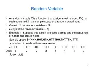
Statistical inference uses impersonal chance to draw conclusions about a population or process based on data drawn from a random sample or randomized experiment.
When data are produced by random sampling or randomized experiment, a statistic is a random variable that obeys the laws of probability.
A sampling distribution shows how a statistic would vary with repeated random sampling of the same size and from the same population. • A sampling distribution, therefore, is a probability distribution of the results of an infinitely large number of such samples.
A population distribution of a random variable is the distribution of its values for all members of the population. • Thus a population distribution is also the probability distribution of the random variable when we choose one individual (i.e. observation or subject) from the population at random.
Recall that a sampling distribution is a conceptual ideal: it helps us to understand the logic of drawing random samples of size-n from the same population in order to obtain statistics by which we make inferences about a parameter. • Population distribution is likewise a conceptual ideal: it tells us that sample statistics are based on probabilities attached to the population from which random samples are drawn.
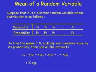
Count: random variable X is a count of the occurrences of some outcome—of some ‘success’ versus a corresponding ‘failure’—in a fixed number of observations. • A count is a discrete random variable that describes categoricaldata (concerning success vs. failure).
Sample proportion: if the number of observations is n, then the sample proportion of observations is X/n. • A sample proportion is also a discrete random variable that describes categorical data (concerning success vs. failure).
Inferential statistics for counts & proportions are premised on a binomial setting.
The Binomial Setting • There are a fixed number n of observations. • The n observations are all independent. • Each observation falls into one of just two categories, which for convenience we call ‘success’ or ‘failure.’ • The probability of a success, p, is the same for each observation. • Strictly speaking, the population must be at least 20 times greater than the sample for counts, 10 times greater for proportions.
Counts • The distribution of the count X of successes in the binomial setting is called the binomial distribution with parameters n & p (i.e. number of observations & probability of success on any one observation). • X is B(n, p)
Finding binomial probabilities: use factorial, binomial table, or software. • Binomial mean & standard deviation:
Example: An experimental study finds that, in a placebo group of 2000 men, 84 got heart attacks, but in a treatment group of another 2000, just 56 got heart attacks. • That is, 2000 independent observations of men have found count X of heart attacks is B(2000, 0.04), so that: . mean=np=(2000)(.04)=80 . sd=sqrt(2000)(.04)(.96)=8.76
Treatment group • . bitesti 2000 56 .04 • N Observed k Expected k Assumed p Observed p • -------------------------------------------------------------------- • 2000 56 80 0.04000 0.02800 • Pr(k >= 56) = 0.998333 (one-sided test) • Pr(k <= 56) = 0.002497 (one-sided test) • Pr(k <= 56 or k >= 106) = 0.005090 (two-sided test) • So, it’s quite unlikely (p=.002) that there would be <=56 heart attacks by chance: the treatment looks promising. What about the placebo group?
Placebo group • . bitesti 2000 84 .04 • N Observed k Expected k Assumed p Observed p • ----------------------------------------------------------------- • 2000 84 80 0.04000 0.04200 • Pr(k >= 84) = 0.339428 (one-sided test) • Pr(k <= 84) = 0.700670 (one-sided test) • Pr(k <= 75 or k >= 84) = 0.647786 (two-sided test) • By contrast, it’s quite likely (p=.70) that the heart attack count in the placebo group would occur by chance. By comparison, then, the treatment looks promising.
Required Sample Size, • Unbiased Estimator • Strictly speaking, he population must be at least 20 times greater than the sample for counts (10 times greater for proportions). • The formula for the binomial mean signifies that np is an unbiased estimator of the population mean.
Binomial test example (pages 370-71): Corinne is a basketball player who makes 75% of her free throws. In a key game, she shoots 12 free throws but makes just 7 of them. What are the chances that she would make 7 or fewer free throws in any sample of 12? • . bitesti 12 7 .75 • N Observed k Expected k Assumed p Observed p • ------------------------------------------------------------------------------- • 12 7 9 0.75000 0.58333 • Pr(k >= 7) = 0.945598 (one-sided test) • Pr(k <= 7) = 0.157644 (one-sided test) • Pr(k <= 7 or k >= 12) = 0.189320 (two-sided test) • Note: ‘bitesti…, detail’ gives k==.103
We’ve just considered sample counts. • Next let’s considered sample proportions.
Sample Proportion • Count of successes in a sample divided by sample size-n. • Whereas a count has whole-number values, a sample proportion is always between 0 & 1.
This is another example of categorical data (success vs. failure). • Mean & standard deviation of a sample proportion:
The population must be at least 10 times greater than the sample. • Formula for a proportion’s mean: unbiased estimator of population mean.
Sample proportion example (pages 373-74): A survey asked a nationwide sample of 2500 adults if they agreed or disagreed that “I like buying new clothes, but shopping is often frustrating & time-consuming.” • Suppose that 60% of all adults would agree with the question. What is the probability that the sample proportion who agree is at least 58%?
How to do it in Stata: . prtesti 2500 .58 .60 One-sample test of proportion x: Number of obs = 2500 Variable Mean Std. Err. [95% Conf. Interval] x .58 .0098712 .5606529 .5993471 P(Z>z) = 0.9794 • That is, there is a 98% probability that the percent of respondents who agree is at least 58%: this is quite consistent with the broader evidence.
We’ve just considered sample proportions. • Next let’s consider sample means.
Sampling Distribution of a Sample Mean • This is an example of quantitative data. • A sample mean is just an average of observations (based on a variable’s expected value). • There are two reasons why sample means are so commonly used:
(1) Averages are less variable than individual observations. (2) Averages are more normally distributed than individual observations.
Sampling distribution of a sample mean • Sampling distribution of a sample mean: if a population has a normal distribution, then the sampling distribution of a sample mean of x for n independent observations will also have a normal distribution. • General fact: any linear combination of independent normal random variables is normally distributed.
Standard deviation of a sample mean: ‘Standard error’ • Divide the standard deviation of the sample mean by the square root of sample size-n. This is the standard error. • Doing so anchors the standard deviation to the sample’s size-n: the sampling distribution of the sample mean across relatively small samples has larger spread & across relatively large samples has smaller spread.
Sampling distribution of a sample mean: If population’s distribution = then the sampling distribution of a sample mean =
Why does the the sampling distribution of the sample mean in relatively small samples have larger spread & in relatively large samples have smaller spread?
Because the standard deviation of the mean is divided by the square root of sample size-n. • So, if you want the sampling distribution of sample means (i.e. the estimate of the population mean)to be less variable, what’s the most basic thing to do?
Make the sample size-n larger. • But there are major costs involved, not only in obtaining a larger sample size per se, but also in the amount of increase needed. • This is because the standard deviation of the sample mean is divided by the square root of n.
What does dividing the mean’s standard deviation by the square root of n imply? • It implies that we’re estimating the variability of the sampling distribution of sample means from the expected value of the population, for an average sample of size n.
In short, we’re using a sample to estimate the population’s standard deviation of the sampling distribution of sample means.
Here’s another principle—one that’s even more important to the sampling distribution of sample means than the Law of Large Numbers.
Central Limit Theorem • As the size of a random sample increases, the sampling distribution of the sample mean gets closer to a normal distribution. • This is true no matter what shape the population distribution has.
The following graphs illustrate the Central Limit Theorem. • The first sample sizes are very small small; the sample sizes become progressively larger.
Note: the Central Limit Theorem applies to the sampling distribution of not only sample means but also sample sums. • Other statistics (e.g., standard deviations) have their own sampling distributions.
The Central Limit Theorem allows us to use normal probability calculations to answer questions about sample means from many observations, even when the population distribution is not normal. • Thus, it justifies reliance of inferential statistics on the normal distribution. • N=30 (but perhaps up to 100 or more, depending on the population’s standard deviation) is a common benchmark threshold for the Central Limit Theorem—although a far larger sample is usually necessary for other statistical reasons. The larger the population’s standard deviation, the larger N must be.
Why not estimate a parameter on the basis of just one observation?
First, because the sample mean is an unbiased estimator of the population mean & is less variable than a single observation. • Recall that averages are less variable than individual observations. • And recall that averages are more normally distributed than individual observations.