3. Random Variables
Explore random variables and probability in experimental outcomes, event determination, and distribution functions in probability theory. Learn about continuous and discrete types of random variables.

3. Random Variables
E N D
Presentation Transcript
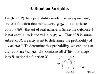
A B 3. Random Variables Let (, F, P) be a probability model for an experiment, and X a function that maps every to a unique point the set of real numbers. Since the outcome is not certain, so is the value Thus if B is some subset of R, we may want to determine the probability of “ ”. To determine this probability, we can look at the set that contains all that maps into B under the function X. Fig. 3.1 PILLAI
Obviously, if the set also belongs to the associated field F, then it is an event and the probability of A is well defined; in that case we can say However, may not always belong to F for all B, thus creating difficulties. The notion of random variable (r.v) makes sure that the inverse mapping always results in an event so that we are able to determine the probability for any Random Variable (r.v):A finite single valued function that maps the set of all experimental outcomes into the set of real numbers R is said to be a r.v, if the set is an event for every x in R. (3-1) PILLAI
Alternatively X is said to be a r.v, if where B represents semi-definite intervals of the form and all other sets that can be constructed from these sets by performing the set operations of union, intersection and negation any number of times. The Borel collection B of such subsets of R is the smallest -field of subsets of R that includes all semi-infinite intervals of the above form. Thus if X is a r.v, then is an event for every x. What about Are they also events ? In fact with since and are events, is an event and hence is also an event. (3-2) PILLAI
Thus, is an event for every n. Consequently is also an event. All events have well defined probability. Thus the probability of the event must depend on x. Denote The role of the subscript X in (3-4) is only to identify the actual r.v. is said to the Probability Distribution Function (PDF) associated with the r.v X. (3-3) (3-4) PILLAI
Distribution Function: Note that a distribution function g(x) is nondecreasing, right-continuous and satisfies i.e., if g(x) is a distribution function, then (i) (ii) if then and (iii) for all x. We need to show that defined in (3-4) satisfies all properties in (3-6). In fact, for any r.v X, (3-5) (3-6) PILLAI
(3-7) (i) and (ii) If then the subset Consequently the event since implies As a result implying that the probability distribution function is nonnegative and monotone nondecreasing. (iii) Let and consider the event since (3-8) (3-9) (3-10) (3-11) PILLAI
using mutually exclusive property of events we get But and hence Thus But the right limit of x, and hence i.e., is right-continuous, justifying all properties of a distribution function. (3-12) (3-13) (3-14) PILLAI
Additional Properties of a PDF (iv) If for some then This follows, since implies is the null set, and for any will be a subset of the null set. (v) We have and since the two events are mutually exclusive, (16) follows. (vi) The events and are mutually exclusive and their union represents the event (3-15) (3-16) (3-17) PILLAI
(vii) Let and From (3-17) or According to (3-14), the limit of as from the right always exists and equals However the left limit value need not equal Thus need not be continuous from the left. At a discontinuity point of the distribution, the left and right limits are different, and from (3-20) (3-18) (3-19) (3-20) (3-21) PILLAI
Fig. 3.2 Thus the only discontinuities of a distribution function are of the jump type, and occur at points where (3-21) is satisfied. These points can always be enumerated as a sequence, and moreover they are at most countable in number. Example 3.1: X is a r.v such that Find Solution: For so that and for so that (Fig.3.2) Example 3.2: Toss a coin. Suppose the r.v X is such that Find PILLAI
Fig.3.3 • Solution: For so that • X is said to be a continuous-type r.v if its distribution function is continuous. In that case for all x, and from (3-21) we get • If is constant except for a finite number of jump discontinuities(piece-wise constant; step-type), then X is said to be a discrete-type r.v. If is such a discontinuity point, then from (3-21) (3-22) PILLAI
From Fig.3.2, at a point of discontinuity we get and from Fig.3.3, Example:3.3 A fair coin is tossed twice, and let the r.v X represent the number of heads. Find Solution: In this case and PILLAI
Fig. 3.4 From Fig.3.4, Probability density function (p.d.f) The derivative of the distribution function is called the probability density function of the r.v X. Thus Since from the monotone-nondecreasing nature of (3-23) (3-24) PILLAI
Fig. 3.5 it follows that for all x. will be a continuous function, if X is a continuous type r.v. However, if X is a discrete type r.v as in (3-22), then its p.d.f has the general form (Fig. 3.5) where represent the jump-discontinuity points in As Fig. 3.5 shows represents a collection of positive discrete masses, and it is known as the probability mass function (p.m.f ) in the discrete case. From (3-23), we also obtain by integration Since (3-26) yields (3-25) (3-26) (3-27) PILLAI
(a) (b) which justifies its name as the density function. Further, from (3-26), we also get (Fig. 3.6b) Thus the area under in the interval represents the probability in (3-28). Often, r.vs are referred by their specific density functions - both in the continuous and discrete cases - and in what follows we shall list a number of them in each category. (3-28) Fig. 3.6 PILLAI
Fig. 3.7 Continuous-type random variables 1. Normal (Gaussian): X is said to be normal or Gaussian r.v, if This is a bell shaped curve, symmetric around the parameter and its distribution function is given by where is often tabulated. Since depends on two parameters and the notation will be used to represent (3-29). (3-29) (3-30) PILLAI
Fig. 3.8 Fig. 3.9 2. Uniform: if (Fig. 3.8) (3.31) 3. Exponential: if (Fig. 3.9) (3-32) PILLAI
4. Gamma: if (Fig. 3.10) If an integer 5. Beta: if (Fig. 3.11) where the Beta function is defined as (3-33) Fig. 3.10 Fig. 3.11 (3-34) (3-35) PILLAI
6. Chi-Square: if (Fig. 3.12) Note that is the same as Gamma 7. Rayleigh: if (Fig. 3.13) 8. Nakagami – m distribution: (3-36) Fig. 3.12 (3-37) Fig. 3.13 (3-38) PILLAI
9. Cauchy: if (Fig. 3.14) 10. Laplace: (Fig. 3.15) 11. Student’s t-distribution with n degrees of freedom (Fig 3.16) (3-39) (3-40) (3-41) Fig. 3.15 Fig. 3.14 Fig. 3.16 PILLAI
12. Fisher’s F-distribution (3-42) PILLAI
Discrete-type random variables 1. Bernoulli: X takes the values (0,1), and 2. Binomial: if (Fig. 3.17) 3. Poisson: if (Fig. 3.18) (3-43) (3-44) (3-45) Fig. 3.18 Fig. 3.17 PILLAI
4. Hypergeometric: 5. Geometric: if 6. Negative Binomial: ~ if 7. Discrete-Uniform: We conclude this lecture with a general distribution due (3-46) (3-47) (3-48) (3-49) PILLAI
to Polya that includes both binomial and hypergeometric as special cases. Polya’s distribution: A box contains a white balls and b black balls. A ball is drawn at random, and it is replaced along with c balls of the same color. If X represents the number of white balls drawn in n such draws, find the probability mass function of X. Solution: Consider the specific sequence of draws where k white balls are first drawn, followed by n – k black balls. The probability of drawing k successive white balls is given by Similarly the probability of drawing k white balls (3-50) PILLAI
followed by n – k black balls is given by Interestingly, pk in (3-51) also represents the probability of drawing k white balls and (n – k) black balls in any other specific order (i.e., The same set of numerator and denominator terms in (3-51) contribute to all other sequences as well.) But there are such distinct mutually exclusive sequences and summing over all of them, we obtain the Polya distribution (probability of getting k white balls in n draws) to be (3-51) (3-52) PILLAI
Both binomial distribution as well as the hypergeometric distribution are special cases of (3-52). For example if draws are done with replacement, then c = 0 and (3-52) simplifies to the binomial distribution where Similarly if the draws are conducted without replacement, Then c = – 1 in (3-52), and it gives (3-53) PILLAI
which represents the hypergeometric distribution. Finally c = +1 gives (replacements are doubled) we shall refer to (3-55) as Polya’s +1 distribution. the general Polya distribution in (3-52) has been used to study the spread of contagious diseases (epidemic modeling). (3-54) (3-55) PILLAI