Ionospheric Research at the Abdus Salam ICTP Aeronomy and Radiopropagation Laboratory

1. Ionospheric Research at the Abdus Salam ICTP Aeronomy and Radiopropagation Laboratory • Sandro M. Radicella • Head, Aeronomy and radiopropagation Laboratory

2. Ionospheric Research at the Abdus Salam ICTPAeronomy and Radiopropagation Laboratory Sandro M. Radicella Head, Aeronomy and Radiopropagation Laboratory

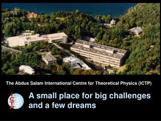
3. The Abdus SalamInternational Centre for Theoretical Physics • Founded in 1964, by the late Nobel Laureate Abdus Salam, receives the majority of its funding from the Italian government and is administered by the United Nations Educational, Scientific and Cultural Organization (UNESCO) and the International Atomic Energy Agency (IAEA).

4. Statistics overview • 4,000 scientists each year • 120 nations • 40 scientific activities per year • 80,000 visits since 1964 • 60% from developing countries • 40% from developed countries

5. Global impact of the Centre • Numbers in red show participations from Developing Countries, • in black participations from • Developed Countries • (to 2001)

6. The Aeronomy and Radiopropagation Laboratory • Aeronomy Section (since 1989): • Research activities: • Ionospheric modeling and effects in satellite positioning • ionospheric scintillations • Wireless Networking Unit: technical support and training in the use of wireless solutions for local area computer networking for academic and research institutions.

7. International activities of the ARPL • Yearly IRI Task Force Activities (since 1994) to discuss topical problems related to the IRI model improvements. • Yearly Schools on the use of radio for digital communications and computer networking • Participation in the European COST 271 Action " Effects of the upper atmosphere on terrestrial and Earth-space communications". • Main contractor of the European Space Agency for the activities of the Ionospheric Expert Team dealing with problems related to global navigation satellite systems. • Since 1999 the ARPL published 17 papers in international journals and 25 in proceedings.

8. Personnel • S. M. Radicella, head • B. Nava • B. Forte • P. Coïsson • C. Fonda • M. Knezevich • G. Miró (EC “Marie Curie” fellow) • Visitors: average of 15 researchers per year • for periods ranging from 1 week to 6 months.

9. An introduction to the ionosphere

10. The vertical profile of electron density in the ionosphere

11. Latitudinal cross section of the ionospheric electron density

12. A bottomside ionogram and profile

13. A topside ionogram and profile

14. Critical frequency and electron density

15. Total electron content • The total electron content (TEC) is the number of electrons in a column of one metre-squared cross-section along a trans-ionospheric path.

16. Total electron content (pictorial)

17. Global map of TEC

18. Trans-ionospheric delay • GPS frequencies • At L1 frequency 1 TECu corresponds to a time delay of 0.54 ns and a range delay of 0.16 m

19. Ionospheric scintillation

20. Ionospheric research at the ARPL

21. Ionospheric modeling • Nequick electron density and TEC model developed for the EGNOS programme of ESA by the Laboratory and the University of Graz (Austria). • Successfully used within the EGNOS End-to-End simulator and been adopted by ITU-R as one of the trans-ionospheric models in Recommendation P.531-5. • The model is proposed for GALILEO single frequency operation in collaboration with the Istituto di Fisica Applicata “Nello Carrara” (former IROE) of Florence, Italy.

22. Steps of a modeling effort • The basic physical approach • The mathematical expressions. • Testing of the model. • Improvements of the model. • Additional testing. • Model validation.

23. Ionospheric effects in satellite positioning • Effects of the ionosphere on satellite positioning on a global scale. • Correction of ionospheric delay using different models in collaboration with groups of Argentina and Spain.

24. Ionospheric scintillations • Evaluation of present experimental techniques for the assessment of scintillation effects in satellite navigation and positioning systems . • Collaboration with research groups from France, Russia, Argentina. New collaboration with groups from Finland and India.

25. A series of models • Electron density profile models originally developed in the framework of the European Commission COST actions 238 and 251. • Based on the original "profiler" proposed by Di Giovanni and Radicella (DGR) give: • electron density on both the bottomside and topside of the ionosphere and • the ionospheric total electron content (TEC). • The models have continuous electron concentration profiles in the function and its first and second derivative.

26. The models • NeQuick, a quick-run model tailored for transionospheric propagation applications (used by the ESA satellite navigation and positioning programs and adopted by Recommendation P.531-6 of the ITU-R as a suitable method for TEC modeling). • COSTprof, a more complex model for ionospheric and plasmaspheric satellite to ground applications (adopted by the European COST 251 action) • NeUoG-plas, a model to be used particularly in assessment studies involving satellite to satellite propagation of radio waves.

27. Physical basis: the Epstein layer • The basic concept is : • a profiler anchored to given points in the real profile

28. The mathematical formulation of NeQuick (1)

29. The mathematical formulation of NeQuick (II)

30. The mathematical formulation of NeQuick (III)

31. NeQuick model input parameters • ITU-R (former CCIR) coefficients for foF2 and M(3000)F2 and R12 and /or monthly mean F 10.7 • Measured values of foE, foF1, foF2 and M(3000)F2 or F2 peak concentration and peak height, • Regional maps of foF2 and M(3000)F2 based on grid values constructed from data obtained at given locations.

32. NeQuick model output parameters • Electron concentration vertical profile to a given height (including the GPS satellite altitude). • Electron concentration along arbitrary ground to satellite or satellite to satellite ray paths. • Vertical Total Electron Content (vTEC) up to any given height. • Slant Total Electron Content between a location on earth and any location in space.

33. NeQuick electron density profiles Nequick electron concentration along arbitrary ground to satellite ray paths for a satellite at 20000 km altitude. Ground location: Lat: 30° N and Long. 10° E, elevation angles 10°, 30°, 60° and 90°.

34. NeQuick global vertical TEC map NeQuick vertical TEC (in TEC units) map using ITU-R coefficients for April, 13 UT and R12 =108.

35. Model comparison with experimental data

36. Comparison of ionospheric effects on point positioning (I) Vertical Components (m) 1  (68 %) 2  (95 %) 3  (99 %) Raw 10.21 17.72 25.97 Klobuchar 7.41 14.20 21.83 NeQuick 6.35 11.04 17.69 Ion Free 3.96 8.31 16.98

37. Comparison of ionospheric effects on point positioning (II) Horizontal Components (m) 1  (68 %) 2  (95 %) 3  (99 %) Raw 3.88 6.07 9.26 Klobuchar 3.93 6.16 9.12 NeQuick 3.58 5.58 8.11 Ion Free 3.31 5.56 8.81

38. An example from our ionospheric scintillations studies

39. Thank you for your attention!