Download
1 / 52
530 likes | 666 Views
Neural Networks. R & G Chapter 8. 8.1 Feed-Forward Neural Networks otherwise known as The Multi-layer Perceptron or The Back-Propagation Neural Network. A diagramatic representation of a Feed-Forward NN. x1=. x2=. y. x3=. Inputs and outputs are numeric. Inputs and outputs.

E N D
Neural Networks. R & G Chapter 8 8.1 Feed-Forward Neural Networks otherwise known as The Multi-layer Perceptron or The Back-Propagation Neural Network
A diagramatic representation of a Feed-Forward NN x1= x2= y x3= Inputs and outputs are numeric. Figure 8.1 A fully connected feed-forward neural network
Inputs and outputs • Must be numeric, but can have any range in general. • However, R &G prefer to consider constraining to (0-1) range inputs and outputs.
Neural Network Input FormatReal input data values are standardized (scaled) so that they all have ranges from 0 – 1. Equation 8.1
Categorical input format • We need a way to convert categores to numberical values. • For “hair-colour” we might have values: red, blond, brown, black, grey. 3 APPROACHES: • 1. Use of (5) Dummy variables (BEST): Let XR=1 if hair-colour = red, 0 otherwise, etc… • 2. Use a binary array: 3 binary inputs can represent 8 numbers. Hence let red = (0,0,0), blond, (0,0,1), etc… However, this sets up a false associations. • 3. VERY BAD: red = 0.0, blond = 0.25, … , grey = 1.0 Converts nominal scale into false interval scale.
Calculating Neuron Output:The neuron threshhold function. The following sigmoid function, called the standard logistic function, is often used to model the effect of a neuron. Consider node i, in the hidden layer. It has inputs x1, x2, and x3, each with a weight-parameter. Then calculate the output from the following function: Equation 8.2
Note: the output values are in the range (0,1). This is fine if we want to use our output to predict a probability of an event happening. . Figure 8.2 The sigmoid function
Other output types • If we have a categorical output with several values, then we can use dummy output notes for each value of the attribute. E.g. if we were predicting one of 5 hair-colour classes, we would have 5 output nodes, with 1 being certain yes, and 0 being certain no.. • If we have a real output variable, with values outside the range (0-1), then another transformation would be needed to get realistic real outputs. Usually the inverse of the scaling transformation. i.e.
Training the Feed-forward net • The performance parameters of the feed-forward neural network are the weights. • The weights have to be varied so that the predicted output is close to the true output value corresponding to the inpute values. • Training of the ANN (Artificial Neural Net) is effected by: • Starting with artibrary wieghts • Presenting the data, instance by instance • adapting the weights according the error for each instance. • Repeating until convergence.
Supervised Learning/Training with Feed-Forward Networks Backpropagation Learning Calculated error of each instance is used to ammend weights. Least squares fitting. All the errors for all instances are squared and summed (=ESS). All weights are then changed to lower the ESS. BOTH METHODS GIVE THE SAME RESULTS. IGNOR THE R & G GENETIC ALGORITHM STUFF.
n r n n’= n + r*(x-n) x Data Instance
8.3 Neural Network Explanation Sensitivity Analysis Average Member Technique
8.4 General Considerations What input attributes will be used to build the network? How will the network output be represented? How many hidden layers should the network contain? How many nodes should there be in each hidden layer? What condition will terminate network training?
Neural Network Strengths Work well with noisy data. Can process numeric and categorical data. Appropriate for applications requiring a time element. Have performed well in several domains. Appropriate for supervised learning and unsupervised clustering.
Weaknesses Lack explanation capabilities. May not provide optimal solutions to problems. Overtraining can be a problem.
Building Neural Networks with iDA Chapter 9
9.1 A Four-Step Approach for Backpropagation Learning Prepare the data to be mined. Define the network architecture. Watch the network train. Read and interpret summary results.
Figure 9.9 Backpropagation learning parameters for the satellite image data
Figure 9.11 Satellite image data: Actual and computed output
Step 1: Prepare The Data To Be Mined The Deer Hunter Dataset
Figure 9.14 Deer hunter data: Unsupervised summary statistics