Download
1 / 25
250 likes | 486 Views
This lecture presents Backstepping controller design for another industrial example, a magnetic levitation train. The control design procedure to be presented in this lecture provides some additional design tools: ( i ) Nonlinear Damping, and (ii) A very simple model based observer design.

E N D
This lecture presents Backstepping controller design for another industrial example, a magnetic levitation train. The control design procedure to be presented in this lecture provides some additional design tools: (i) Nonlinear Damping, and (ii) A very simple model based observer design. ECE 893 Industrial Applications of Nonlinear Control Dr. UgurHasirciClemson University, Electrical and Computer Engineering Department Spring 2013
Before the design, I would like to remind that the experimental setup is ready to test. By using the guide posted at course website, please install the software set, make the required laptop configuration, and then go to Riggs 25 (passcode is 1495#). • At workstation 3, you will find the experimental setup. Connect the ethernet cable to your laptop (host computer), launch xPC Target Explorer, upload analog_loopback.mdl file, build it, and run the model. • As you remember, this mdl file sends a sin signal to the Quanser Q4 analog output port. If you see a sin wave at the target PC monitor, then all your installations are ok ! ECE 893 Industrial Applications of Nonlinear Control Dr. UgurHasirciClemson University, Electrical and Computer Engineering Department Spring 2013
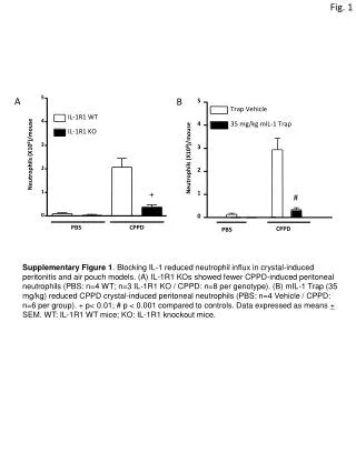
Magnetic levitation (maglev) trains present a powerful alternative to land, air, and classical rail transportation systems. Because of the friction between wheel and rail, conventional trains have speed limitations, operate at high noise levels and require frequent maintenance. Maglev trains replace wheel by electromagnets and produce the propulsion force without any contact. This motivates researchers to investigate some novel maglev topologies to increase the ride quality and to decrease the cost of the overall system. ECE 893 Industrial Applications of Nonlinear Control Dr. UgurHasirciClemson University, Electrical and Computer Engineering Department Spring 2013
A novel topology for maglev systems was patented by Levi and Zabar. This system uses only one air-cored tubular linear induction motor to produce levitation, propulsion and guidance forces simultaneously . • Specifically, we design, implement, test and controlthe newly proposed maglev system in this study. Main aim of the study is to prove that the experimental performance of this maglev system is satisfactory to use it in a commercial application. ECE 893 Industrial Applications of Nonlinear Control Dr. UgurHasirciClemson University, Electrical and Computer Engineering Department Spring 2013
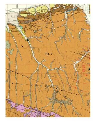
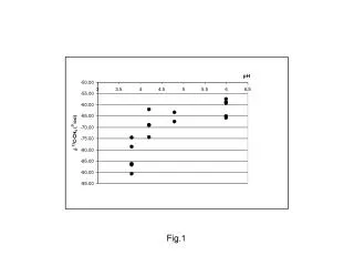
The motor has two main parts as in a classical rotary induction motor: the primary; which consists of the drive coils, and the secondary; which consists of an aluminum slit sleeve. Drive coils can be placed either on the track or onboard the vehicle. Fig. 1 shows the proposed maglev system with energization from the wayside, and Fig. 2 shows the other configuration of the proposed system with energization onboard the vehicle. ECE 893 Industrial Applications of Nonlinear Control Dr. UgurHasirciClemson University, Electrical and Computer Engineering Department Spring 2013 Fig. 2. Proposed maglev system with energization onboard the vehicle. (1-vehicle, 2-drive coils, 3-aluminum sleeve, 4-support) Fig. 1. Proposed maglev system with energizationfrom the wayside. (1-vehicle, 2-drive coils, 3-aluminum sleeve, 4-support)
Mechatronics Forum Dr. Ugur HasirciClemson University, Electrical and Computer Engineering Department Spring 2013 • Main Advantages: • This new system produces levitation, propulsion and guidance forces simultaneously by using only one motor. • It is not needed to control the levitation and guidance forces because the restoring force centers the moving part, as will be proved experimentally in the following. ECE 893 Industrial Applications of Nonlinear Control Dr. UgurHasirciClemson University, Electrical and Computer Engineering Department Spring 2013
Mechatronics Forum Dr. UgurHasirciClemson University, Electrical and Computer Engineering Department Spring 2013 ECE 893 Industrial Applications of Nonlinear Control Dr. UgurHasirciClemson University, Electrical and Computer Engineering Department Spring 2013 Entire System Acceleration Sensor Drive Coils
ECE 893 Industrial Applications of Nonlinear Control Dr. UgurHasirciClemson University, Electrical and Computer Engineering Department Spring 2013
ECE 893 Industrial Applications of Nonlinear Control Dr. UgurHasirciClemson University, Electrical and Computer Engineering Department Spring 2013
ECE 893 Industrial Applications of Nonlinear Control Dr. UgurHasirciClemson University, Electrical and Computer Engineering Department Spring 2013
ECE 893 Industrial Applications of Nonlinear Control Dr. UgurHasirciClemson University, Electrical and Computer Engineering Department Spring 2013
State-Space Model ECE 893 Industrial Applications of Nonlinear Control Dr. UgurHasirciClemson University, Electrical and Computer Engineering Department Spring 2013 where ids and iqs are stator current components on d and q-axis, λds and λqs depict rotor flux components on d and q-axis, V is linear velocity, Rs is stator resistance per phase, Ls and Lrrepresent stator and rotor inductances per phase,Lmis magnetizing inductance per phase, pdenotes number of poles, h is pole pitch, σdepicts leakage coefficient, Tr is rotor time constant, Kf represents force constant, FL depicts load force, M is the total mass of the moving part, Bdenotes viscous friction coefficient, and finally, Vd and Vq are stator voltages on d and q-axis.
To simplify the control design procedure, system dynamics given can be written in a more compact form as ECE 893 Industrial Applications of Nonlinear Control Dr. UgurHasirciClemson University, Electrical and Computer Engineering Department Spring 2013 Control problem can be defined as follow; drive the linear velocity x5 to a desired velocity profile x5d while the rotor flux components x3and x4 are unmeasurable. It is assumed that all parameters related electrical and mechanical subsystems are known. To determine the performance of the controller to be designed, an error signal can be defined as
Due to the states x3 and x4 (rotor flux components) are unmeasurable, let design a model based observer as Observer ECE 893 Industrial Applications of Nonlinear Control Dr. UgurHasirciClemson University, Electrical and Computer Engineering Department Spring 2013 where and are the estimates of unmeasurable states, x3 and x4. Define the state estimation errors as This implies the state estimation error system will be
To show the stability of this observer, following Lyapunov function can be used: ECE 893 Industrial Applications of Nonlinear Control Dr. UgurHasirciClemson University, Electrical and Computer Engineering Department Spring 2013 State estimation errors go to zero exponentially, and thus we can use estimated values of this unmeasurable states during the control design. ■
By going back to the control design, we investigate the error system dynamics; If x3 and x4 were available for measurement, one could choose the produced electromechanical force Fe=c2(x1x4-x2x3) as the virtual control input and initiate directly the backstepping procedure. Since these state variables are not measured but estimated, observer backsteppingshould be applied. ECE 893 Industrial Applications of Nonlinear Control Dr. UgurHasirciClemson University, Electrical and Computer Engineering Department Spring 2013 Nonlinear Damping Term The nonlinear damping term defined as where d1 is the damping coefficient, will be used to damp the state estimation errors and while designing the control input signals.
In this step, a new error variable (a new coordinate) is defined as Then the final expression for the error system dynamics will be ECE 893 Industrial Applications of Nonlinear Control Dr. UgurHasirciClemson University, Electrical and Computer Engineering Department Spring 2013 By following the standard backstepping procedure, let’s backstep on z1. To reach the control input signals u1 and u2, dynamics of z1 must be investigated. Note that z1 is a function of and . By using the partial differentiation, the expression for z1 dynamics is obtained as where are the factors of related signals which contain all measurable states and known parameters. For simplicity, their explicit expressions are written here due to their length. Then the feedback rule is where d2 is the second damping coefficient and Kz1 is a control gain. If control inputs are designed as above, the final dynamics for z1 will be
A very important subtask in meeting the control objective is to ensure a bounded rotor flux, i.e., rotor flux should be forced to track a bounded signal. Since x3 and x4 are not measurable, we replace them by their estimates and define a new error variable as ECE 893 Industrial Applications of Nonlinear Control Dr. UgurHasirciClemson University, Electrical and Computer Engineering Department Spring 2013 where ψd is the desired flux. Investigating ε dynamics yields Once again, we have to choose a virtual control input. One should select the term as virtual control input, then add and subtract a second stabilizing function α2 to the right hand side of above equation as shown in the following.
ECE 893 Industrial Applications of Nonlinear Control Dr. UgurHasirciClemson University, Electrical and Computer Engineering Department Spring 2013 By combining two expressions for control input signals, which are we can write the control input signal in vector matrix form as
The designed control law is well defined if the matrix ECE 893 Industrial Applications of Nonlinear Control Dr. UgurHasirciClemson University, Electrical and Computer Engineering Department Spring 2013 is globally invertible. Before presenting the stability analysis, let me remind the final dynamics of all error variables. We will need them to complete the stability analysis.
To show the stability of the overall system, let’s select the Lyapunov function as follows: ECE 893 Industrial Applications of Nonlinear Control Dr. UgurHasirciClemson University, Electrical and Computer Engineering Department Spring 2013 Why do we add this term to the final Lyapunov function? We already showed the exponential stability of the observation errors !!! The answer is hidden in another characteristic behavior of the nonlinear systems: ------------- FINITE ESCAPE TIME -------------- Please see the following side note, which is a well-known demonstration of Finite Escape Time.
Consider the system where is the observation error for unmeasurable state of the system, . Assume that we already showed the observation error goes to zero exponentially, i.e., ECE 893 Industrial Applications of Nonlinear Control Dr. UgurHasirciClemson University, Electrical and Computer Engineering Department Spring 2013 Then the solution of the differential equation is which escape to infinity in a finite time, which is Consequently, even though the observer is exponentially stable, the overall system might become unstable in nonlinear systems. This is the reason to put the observation errors into the final Lyapunov function, and also to use Nonlinear Damping terms in the design, to damp the terms related observation errors. !!!!!! ■
Back to the stability analysis: ECE 893 Industrial Applications of Nonlinear Control Dr. UgurHasirciClemson University, Electrical and Computer Engineering Department Spring 2013 GAS of the E.P. is achieved.
Tracking Error ECE 893 Industrial Applications of Nonlinear Control Dr. UgurHasirciClemson University, Electrical and Computer Engineering Department Spring 2013
Your guns before today ECE 893 Industrial Applications of Nonlinear Control Dr. UgurHasirciClemson University, Electrical and Computer Engineering Department Spring 2013 Backstepping Your guns as of today Backstepping Nonlinear Damping You will have lots of guns at the end of the semester to control the systems in nature.