Algorithms Analysis lecture 11 Greedy Algorithms
Algorithms Analysis lecture 11 Greedy Algorithms. Greedy Algorithms. Activity Selection Problem Knapsack Problem Huffman Problem. Greedy Algorithms. Similar to dynamic programming, but simpler approach Also used for optimization problems

Algorithms Analysis lecture 11 Greedy Algorithms
E N D
Presentation Transcript
Greedy Algorithms • Activity Selection Problem • Knapsack Problem • Huffman Problem
Greedy Algorithms • Similar to dynamic programming, but simpler approach • Also used for optimization problems • Idea: Make a locally optimal choice in hope of getting a globally optimal solution
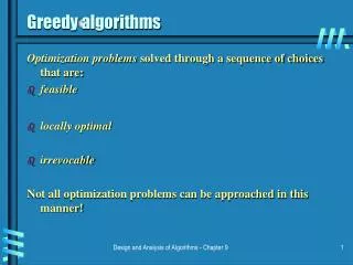
Greedy Algorithms For optimization problems Dynamic programming determine the best choices is overkill Greedy algorithm makes the choice that looks best at the moment in order to get optimal solution. Optimistic متفائل Almost always but do not always yield optimal solutions. We will have the Activity selection example and we will solve it using both algorithms
Activity Selection • Schedule nactivities that require exclusive use of a common resource S = {a1, . . . , an}– set of activities • ai needs resource during period [si , fi) • si= start time and fi = finish time of activity ai • 0 si < fi < • Activities ai and aj are compatible if the intervals [si , fi) and [sj, fj) do not overlap fi sj fj si i j j i
Activity Selection Problem Select the largest possible set of non- overlapping (mutually compatible) activities. E.g.: • Activities are sorted in increasing order of finish times • A subset of mutually compatible activities: {a3, a9, a11} • sets of mutually compatible activities: {a1, a4, a8, a11} and {a2, a4, a9, a11}
Optimal Substructure, step 1 • Define the space of subproblems: Sij = { ak S : fi ≤ sk < fk ≤ sj } • activities that start after ai finishes and finish before aj starts
Representing the Problem, step 1 • Range for Sij is 0 i, j n + 1 • In a set Sij we assume that activities are sorted in increasing order of finish times: f0 f1 f2 … fn < fn+1 • What happens if i ≥ j ? • For an activity ak Sij: fi sk < fk sj < fj contradiction with fi fj! Sij = (the set Sij must be empty!) • We only need to consider sets Sij with 0 i < j n + 1
Sij Skj Sik Optimal Substructure, step 1 • Subproblem: • Select a maximum size subset of mutually compatible activities from set Sij • Assume that a solution to the above subproblem includes activity ak (Sij is non-empty) Solution to Sij = (Solution to Sik) {ak} (Solution to Skj) Solution to Sij = Solution to Sik + 1 + Solution to Skj
Aij Akj Aik Optimal Substructure (cont.) Suppose Aij = Optimal solution to Sij • Claim: Sets Aik and Akj must be optimal solutions • Assume Aik’ that includes more activities than Aik Size[Aij’] = Size[Aik’] + 1 + Size[Akj] > Size[Aij] Contradiction: we assumed that Aij is the maximum # of activities taken from Sij
Recursive Solution, step 2 • Any optimal solution (associated with a set Sij) contains within it optimal solutions to subproblems Sik and Skj • c[i, j] = size of maximum-size subset of mutually compatible activities in Sij • If Sij = c[i, j] = 0 (i ≥ j)
Sij Skj Sik Recursive Solution, step 2 If Sij and if we consider that ak is used in an optimal solution (maximum-size subset of mutually compatible activities of Sij) c[i, j] = c[i,k] + c[k, j] + 1
Recursive Solution, step 2 0 if Sij = c[i, j] = max {c[i,k] + c[k, j] + 1} if Sij • There are j – i – 1 possible values for k • k = i+1, …, j – 1 • ak cannot be ai or aj (from the definition of Sij) Sij = { ak S : fi ≤ sk < fk ≤ sj } • We check all the values and take the best one We could now write a tabular, bottom-up dynamic programming algorithm i < k < j ak Sij
Theorem Let Sij and am be the activity in Sij with the earliest finish time: fm = min { fk: ak Sij } Then: • am is used in some maximum-size subset of mutually compatible activities of Sij • There exists some optimal solution that contains am • Sim = • Choosing am leaves Smj the only non-empty subproblem
Smj Sim Proof • Assume ak Sim fi sk < fk sm < fm fk < fm contradiction ! am did not have the earliest finish time There is no ak Sim Sim = Sij sm fm ak am
sm fm am fk Greedy Choice Property Proof • am is used in some maximum-size subset of mutually compatible activities of Sij • Aij = optimal solution for activity selection from Sij • Order activities in Aij in increasing order of finish time • Let ak be the first activity in Aij = {ak, …} • If ak = am Done! • Otherwise, replace ak with am (resulting in a set Aij’) • since fm fk the activities in Aij’ will continue to be compatible • Aij’ will have the same size with Aij am is used in some maximum-size subset Sij
Why is the Theorem Useful? • Making the greedy choice (the activity with the earliest finish time in Sij) • Reduce the number of subproblems and choices • Solve each subproblem in a top-down fashion 2 subproblems: Sik, Skj 1 subproblem: Smj Sim = 1 choice: the activity with the earliest finish time in Sij j – i – 1 choices
Greedy Approach • To select a maximum size subset of mutually compatible activities from set Sij: • Choose am Sij with earliest finish time (greedy choice) • Add am to the set of activities used in the optimal solution • Solve the same problem for the set Smj • From the theorem • By choosing am we are guaranteed to have used an activity included in an optimal solution We do not need to solve the subproblem Smj before making the choice! • The problem has the GREEDY CHOICE property
Characterizing the Subproblems • The original problem: find the maximum subset of mutually compatible activities for S = S0, n+1 • Activities are sorted by increasing finish time a0, a1, a2, a3, …, an+1 • We always choose an activity with the earliest finish time • Greedy choice maximizes the unscheduled time remaining • Finish time of activities selected is strictly increasing
am fm am fm am fm A Recursive Greedy Algorithm Alg.: REC-ACT-SEL (s, f, i, j) • m ← i + 1 • while m < jandsm < fi ►Find first activity in Sij • do m ← m + 1 • if m < j • then return {am} REC-ACT-SEL(s, f, m, j) • else return • Activities are ordered in increasing order of finish time • Running time: (n)– each activity is examined only once • Initial call: REC-ACT-SEL(s, f, 0, n+1) ai fi
k sk fk Example a1 m=1 a0 a2 a3 a1 a4 m=4 a1 a5 a4 a1 a6 a1 a4 a1 a7 a1 a4 a8 m=8 a4 a1 a9 a4 a1 a8 a10 a4 a8 a1 a11 m=11 a4 a1 a8 a11 a4 a8 a1 0 6 9 11 1 2 3 4 5 7 8 10 12 13 14
An Iterative Greedy Algorithm am fm am fm Alg.: GREEDY-ACTIVITY-SELECTOR(s, f) • n ← length[s] • A ← {a1} • i ← 1 • for m ← 2to n • do if sm ≥ fi ► activity am is compatible with ai • then A ← A {am} • i ← m ► ai is most recent addition to A • return A • Assumes that activities are ordered in increasing order of finish time • Running time: (n)– each activity is examined only once am fm ai fi
Activity Selection B (1) C (2) A (3) E (4) D (5) F (6) G (7) H (8) Time 0 1 2 3 4 5 6 7 8 9 10 11 0 1 2 3 4 5 6 7 8 9 10 11
Activity Selection B (1) C (2) A (3) E (4) D (5) F (6) G (7) H (8) Time 0 1 2 3 4 5 6 7 8 9 10 11 B 0 1 2 3 4 5 6 7 8 9 10 11
Activity Selection B (1) C (2) C (2) A (3) E (4) D (5) F (6) G (7) H (8) Time 0 1 2 3 4 5 6 7 8 9 10 11 B E H 0 1 2 3 4 5 6 7 8 9 10 11
Steps Toward Our Greedy Solution • Determine the optimal substructure of the problem • Develop a recursive solution • Prove that one of the optimal choices is the greedy choice • Show that all but one of the subproblems resulted by making the greedy choice are empty • Develop a recursive algorithm that implements the greedy strategy • Convert the recursive algorithm to an iterative one
Another Example : The Knapsack Problem- two version • The 0-1 knapsack problem • A thief robbing a store finds n items: the i-th item is worth vi dollars and weights wi pounds (vi, wi integers) • The thief can only carry W pounds in his knapsack • Items must be taken entirely(1) or left behind (0) • Which items should the thief take to maximize the value of his load? • The fractional knapsack problem • Similar to above • The thief can take fractions of items
The 0-1 Knapsack Problem • Thief has a knapsack of capacity W • There are n items: for i-th item value vi and weight wi • Goal: • find xi such that for all xi = {0, 1}, i = 1, 2, .., n wixi W and xivi is maximum
50 30 $120 + 20 $100 $220 0-1 Knapsack - Greedy Strategy 50 50 • E.g.: Item 3 30 20 Item 2 $100 + 20 Item 1 10 10 $60 $60 $100 $120 $160 $6/pound $5/pound $4/pound • None of the solutions involving the greedy choice (item 1) leads to an optimal solution • The greedy choice property does not hold
0-1 Knapsack - Dynamic Programming • P(i, w)– the maximum profit ربح that can be obtained from items 1 to i, if the knapsack has size w • Case 1: thief takes item i P(i, w) = • Case 2: thief does not take item i P(i, w) = vi + P(i - 1, w-wi) P(i - 1, w)
Optimal Substructure • Consider the most valuable load that weights at most W pounds • If we remove item j from this load • The remaining load must be the most valuable load weighing at most W – wjthat can be taken from the remaining n – 1 items
Fractional Knapsack Problem • Knapsack capacity: W • There are n items: the i-th item has value vi and weight wi • Goal: • find xi such that for all 0 xi 1, i = 1, 2, .., n wixi W and xivi is maximum
Fractional Knapsack Problem Greedy strategy : • Pick the item with the maximum value per pound vi/wi • If the supply of that element is exhausted and the thief can carry more: take as much as possible from the item with the next greatest value per pound • It is good to order items based on their value per pound
Fractional Knapsack Problem Alg.:Fractional-Knapsack (W, v[n], w[n]) • While w > 0 and as long as there are items remaining • pick item with maximum vi/wi • remove item i from list • w w – xiwi • w– the amount of space remaining in the knapsack (w = W) • Running time: (n) if items already ordered; else (nlgn)
Fractional Knapsack - Example 20 --- 30 50 50 • E.g.: $80 + Item 3 30 20 Item 2 $100 + 20 Item 1 10 10 $60 $60 $100 $120 $240 $6/pound $5/pound $4/pound
Huffman Code Problem Huffman’s algorithm achieves data compression by finding the best variable length binary encoding scheme for the symbols that occur in the file to be compressed.
Huffman Code Problem • The more frequent a symbol occurs, the shorter should be the Huffman binary word representing it. • The Huffman code is a prefix-free code. No prefix of a code word is equal to another codeword.
C: Alphabet Overview • Huffman codes: compressing data (savings of 20% to 90%) • Huffman’s greedy algorithm uses a table of the frequencies of occurrence of each character to build up an optimal way of representing each character as a binary string
Example Assume we are given a data file that contains only 6 symbols, namely a, b, c, d, e, f With the following frequency table: Find a variable length prefix-free encoding scheme that compresses this data file as much as possible?
Huffman Code Problem •Left tree represents a fixed length encoding scheme •Right tree represents a Huffman encoding scheme
Constructing A Huffman Code Total computation time = O(n lg n) O(lg n) O(lg n) O(lg n) O(lg n)
Cost of a Tree T • For each character c in the alphabet C • let f(c) be the frequency of c in the file • let dT(c) be the depth of c in the tree • It is also the length of the codeword. Why? • Let B(T) be the number of bits required to encode the file (called the cost of T)