Download
1 / 47
520 likes | 972 Views
ST 370 Probability and Statistics for Engineers Lecture 3 Descriptive Statistics. Dr. Zhao-Bang Zeng Department of Statistics NC State University. Outline for Today’s Talk. Numerical Descriptive Statistics Graphical Descriptive Statistics. Numerical Descriptive Statistics. Mean Median

E N D
ST 370 Probability and Statistics for Engineers Lecture 3 Descriptive Statistics Dr. Zhao-Bang Zeng Department of Statistics NC State University
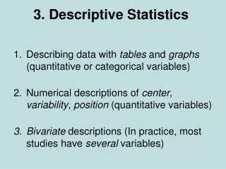
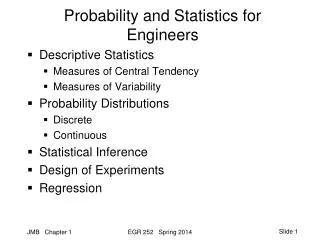
Outline for Today’s Talk • Numerical Descriptive Statistics • Graphical Descriptive Statistics
Numerical Descriptive Statistics • Mean • Median • Mode • Variance • Standard Deviation • Quartiles
Mean, Median and Mode • Mean = Average value Let n denote the sample size: • (Sample) Mean - Average of all n observations • (Sample) Median • The middle observation if n is odd • The average of the 2 middle observations if n is even. • (Sample) Mode – most common observation
Mean, Median and Mode • The mean is more sensitive to extreme values than the median. • The relationship between the mean and the median can be used to determine the shape of the distribution of data.
Mean, Median and Mode • For symmetric distributions: mean = median = mode • For positively skewed distributions: mean > median • For negatively skewed distributions: mean < median
Mean, Median and Mode: Which measure to use? • The choice depends on the shape of the distribution, the type of data and the purpose of your study • Skewed: median • Categorical: mode • Total quantity: mean
Mean and Median • Consider the means of two data sets with the same median {5, 8, 9, 10, 11} vs {5, 8, 9, 10, 68}
Sample Variance and Standard Deviation • Let be the mean of a sample x1,…,xn: The (sample) variance is given by • The (sample) standard deviation s is the non-negative square root of the variance.
Sample Variance and Standard Deviation • If observed values are far apart, the variance and standard deviation will be relatively large • Variance and standard deviation are strongly affected by outliers
Sample Variance and Standard Deviation • Note that variance and standard deviation are greater than or equal to zero. They are only zero when all the observed values are equal • If we multiply all of the numbers in the data set by a non-zero constant c, the effect is to • multiply the variance by the square of c • multiply the standard deviation by c
Empirical Rule • If the data are symmetric, we can use the Empirical Rule (or 68-95-99.7 rule) as an approximation • Roughly 68% of the data fall within one standard deviation of the mean • Roughly 95% of the data fall within two standard deviations of the mean • Roughly 99.7 % of the data fall within three standard deviations of the mean Note: These numbers come from normal distribution theory, which we’ll see later
Ex. Empirical Rule • Assume that we have a symmetric data set with = 515 and s =114. Then, • Roughly 68% of the data fall between [401, 629] • Roughly 95% of the data fall between [287, 743] • Roughly 99.7% (almost all) of the data fall between [173, 857]
Why do we compute variation? • Two basketball players with the same shooting percentage may be very different in terms of consistency. • Two companies may have the same average salary, but very different distributions. • Thus we need to know the spread, or the variability of the values.
Quartiles • Q1 = Q(.25) is the 1st (lower) quartile. • Q2 = Q(.50) is the median. • Q3 = Q(.75) is the 3rd (upper) quartile.
Quartiles • Q1 is the median of the ordered observations that lie to the left of Q2. • Q3 is the median of the ordered observations that lie to the right of Q2. • Interquartile Range (IQR) - gives the spread of the middle 50% of the data. IQR = Q3 – Q1
Quartiles • Order the data from smallest to largest 56, 67, 68, 72, 74, 75, 88, 90, 97, 99 • The median splits the data into two parts. We want the same amount of observations on both sides of the median. Any point between 74 and 75 would serve the purpose. As a convention, we take the average of the two (74+75)/2=74.5 as the median.
Quartiles Ex. 56, 67, 68, 72, 74, 75, 88, 90, 97, 99 • There are different conventions for finding quartiles! We choose to use the following convention:To find Q1 and Q3, find the median of the two halves of the data formed as determined by Q2 • So Q1 = 68; Q3 = 90
Quartiles Ex. 56, 67, 68, 72, 74, 75, 88, 90, 97, 99,100 • If the number of data points n is odd then our convention is that Q2 is counted as part of the lower half and upper half • Q2=75; Q1=(68+72)/2=70 ; Q3=(90+97)/2=93.5
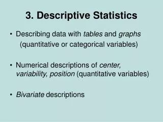
Graphical Descriptive Statistics • Histograms • Box plots
Histograms • The most common graphical summary of quantitative data is a histogram • Describes the observed distribution of a single quantitative variable • Graphs the frequencies or relative frequencies of a single quantitative variable
Histograms (how?) • Choose intervals (or bins) that cover the entire range of the data • Count the number of observations per interval • Draw rectangles with heights corresponding to the number in interval • Note: for relative frequency histogram, the height is relative frequency for each interval
Histograms (How?) • Intervals must be non-overlapping • Typically, an observation equal to a boundary value is put in the higher interval. • Intervals must be contiguous (rectangles touch each other) • Intervals must be of equal width • Often we choose “nice” boundaries
Histograms (How?) • For discrete data, center the interval about the data point • Too many classes will spread the data out, thereby not revealing the pattern. Too few classes will lump the data. • We typically want the number of classes to be between 5 and 20. • When the data set is small, we want fewer classes • When the data set is large, we want more classes • The height of the bar gives the frequency or relative frequency
Things to look for in a histogram • Shape • Location • Spread
Things to look for in a histogram: Shape • How many modes (or peaks) are there • Unimodal: one peak • Bimodal: two peaks
The modal class A unimodal histogram
A modal class A modal class A bimodal histogram
Things to look for in a histogram: Shape • Symmetric: • histogram in which the right half is a mirror image of the left half (bell-shaped) • Skewed to the right: • histogram in which the right tail is more stretched out than the left (long tail to the right) • Skewed to the left: • histogram in which the left tail is more stretched out than the right (long tail to the left)
Skewness Left skewed Right skewed
Examples of variables with a skewed distribution • Income (typically skewed to the right) • Exam scores (skewed to the left)
Things to look for in a histogram: Location • Location - measures of central tendency (Where is the middle of the data?) • It can be difficult to describe the central location when the data are skewed.
Mode Mean Median Mean Mode Median Things to look for in a histogram: Location • For symmetric distributions, mean = median = mode • For skewed distributions, the three measures differ.
Things to look for in a histogram: Spread • How spread out are the data? • If all observations are between a and b, then the range is b-a. • Are there outliers? (unusually large or small observations)
Determining the median for a given histogram • Add the heights of the rectangles to determine n (n=75) • Median Q2 is located at position 38 • Add up the rectangle heights starting from the left until reaching 38. • May not be able to determine exact value (From statcrunch: median Q2=90)
Boxplots • Boxplots give less detail than a histogram • First step : obtain 5-number summary min Q1 Q2 Q3 max • Q1, Q2 (median) and Q3 are quartiles (they divide the data into four parts)
Drawing the box • Can be drawn vertically or horizontally • Box ends are at Q1 and Q3 • Length of box (Q3-Q1) is the interquartile range (IQR) • Place a line across the box at the median • Upper fence placed at Q3+1.5 IQR, lower fence Q1-1.5 IQR • Whiskers are drawn to the “last” actual data value within the fences (might be min or max) • May need to indicate outliers with individual data points (some books uses asterisks) Salary of CEOs (thousands $)
Reading boxplots • Displays the 5-number summary • Symmetric data: Q2 is in the middle of the box, with symmetric whiskers • Right skewed data: longer right (top) whisker and the median towards the left (bottom) of the box • Left skewed data: longer left (bottom) whisker and the median towards the right (top) of the box Life Expectancy
Reading boxplots • Possible measure of the center of the data from a boxplot: median • Possible measures of spread from a boxplot: range (max-min), IQR (Q3-Q1)
Final Thoughts: Handling Outliers • Detect them using graphical and numerical methods. • Check the data to make sure an entry is correct. • To reduce influence of outlier • delete the observation (BE CAREFUL!) • Use transformations, robust methods (median as measure of spread)