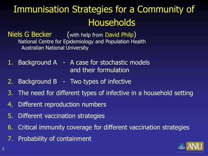
Immunisation Strategies for a Community of Households

1. Immunisation Strategies for a Community of Households Niels G Becker (with help fromDavid Philp)National Centre for Epidemiology and Population Health Australian National University • Background A - A case for stochastic models and their formulation • Background B - Two types of infective • The need for different types of infective in a household setting • Different reproduction numbers • Different vaccination strategies • Critical immunity coverage for different vaccination strategies • Probability of containment

2. Background A • A case for stochastic models • The deterministic SIR model has some limitations • It and Stare taken as continuous when they are really integers. (Of concern when either is small) • They suggest that an outbreak always takes off when • R0 s0> 1. (Not always the case.) • They ignore the chance element in transmission. • (Of particular concern when Itor St are small, • e.g. during the early stages, or when control is effective)

3. Formulation of stochastic infectious disease models When we allow for chance, the description of disease transmission involves a probability distribution for the number of infectives and susceptibles at each point in time. Equations for these distributions are easy to write down, but difficult to solve. With the speed of modern computers stochastic formulations are often accommodated by simulation studies. That is, many realisations of the random process are generated, from which means and proportions are calculated.

4. Some questionscan be explored analytically, including: • What is the probability that an imported infection leads to a major outbreak? • What fraction of the community needs to be immune to ensure that an imported infection can not lead to a major outbreak? • What is the distribution of the eventual size of the outbreak?

5. Branching processes are a central tool in such analyses A standard Branching Process (BP) is a population model in which each individual independently generates a number of offspring. This number is randomly selected from a common probability distribution. Some of results in the rich theory of Branching Processes are useful for studying the control of outbreaks of an infectious disease. In disease transmission a BP is used to approximate the population dynamics of infectives, while the depletion of susceptibles remains negligible. This applies during the early stages of an outbreak initiated by an imported infection and for the entire outbreak when the outbreak is minor.

6. Early stages of an outbreak Generation Mean of offspring distribution = µ Mean number in generation r = I0 µ r

7. and after that … Generation

8. Some results from Branching Processes: • Suppose the mean of the offspring distribution is µ. • The BP becomes extinct with probability 1 when µ< 1. • The mean of the offspring distribution for infectives is µ (1-v), when a fraction v of close contacts is with immune people. • The BP becomes extinct with probability 1 when µ (1-v) < 1. • Therefore, the critical immunity coverage is 1 – 1/ µ. • Let X be the number of offspring an infective has. • Suppose that Pr(X = r) = pr • The probability that 1 infective starts an outbreak that does • not take off is • p0 + p1 p0 + p1 p1 p0 + p2 p0 p0+ etc, etc, etc

9. A simpler approach: • Let q be the probability that an outbreak started by 1 infective does not take off. • If the first infective has x offspring then each of them starts an independent BP and the probability that none of those x BPs takes off is q x. • Therefore q = p0.1 + p1.q + p2.q2 + p3.q3 + … • So q is the smallest solution of • s = φ(s), • where φ is the probability generating function of the offspring distribution.

10. Illustration • Consider the Poisson offspring distribution with mean (1-v), where v is the fraction immune. • The p.g.f. is then φ(s) = exp[ (1-v)(s-1)] • With  = 3, we need to fix vand solve • s = exp[3(1-v)(s-1)] • The value v that achieves q is v= 1 – ln(q) /[3(q -1)] q v

11. Background B • Different types of infective • Suppose there are two types of individual, perhaps children and adults, who differ in susceptibility and infectivity, and mix differently. • Now each type has a different offspring distribution. • Means are again central for determining interventions that can contain transmission, BUT we need a mean matrix.

12. Mean matrix (with everyone susceptible): Result from multi-type Branching Processes: A multi-type branching process becomes extinct with probability 1 if the largest eigenvalue of the mean matrix is less than 1. For the above matrix: R = larger root of (4-x)(1-x)-2*2=0, that is R= 5. Is this a “reproduction” number?

13. If the branching process takes off, then eventually infectives will consist of 2/3 children and 1/3 adults. [Obtain this from the eigenvector corresponding to eigenvalue 5] If, at that stage, we sample an infective at random, then the mean number of offspring is (2/3)*6 + (1/3)*3 =5 so R is a reproduction number in that sense. It is the eventual rate of growth of the BP. While this ‘reproduction number’ is a useful tool for determining the requirements for containment, its interpretation does not really provide a lot of direct insights for infectious disease epidemiology.

14. Suppose we immunise a fraction vc of children and a fraction va of adults. Then the mean matrix becomes This changes the reproduction number to the larger root of [4(1-vc) –x][(1-va) –x]- 4(1-vc)(1-va) =0. Thus Rv= 5 – va – 4vc. Can now address questions such as: 1. What is the smallest coverage required to make Rv< 1? ` 2. What is the critical coverage whenva = vc?

15. Household structure Choice of Reproduction Number There are numerous ways to define a reproduction number for transmission in a community of households. Becker and Dietz (1996) define 4 reproduction numbers assuming an SIR model and that the community consists of households of size 3. These reproduction numbers are distinguished by the way infections are attributed to infectives. To illustrate the choice we define here 2 reproduction numbers in the simplest setting, where all households have size 2.

16. RI0 reproduction based on individuals infectedFor this reproduction number we attribute cases actually infected A For calculating RI0 we attribute 4 infections to A, in this example.

17. A primary case in a household of two can infect community members AND their household partner. A secondary case in a household of two can infect only community members. Their potential to infect others differs, so consider them as different types of infective, P and S.

18. On average, a primary case infects  individuals outside the household and pindividuals within the household.On average, a secondary case infects  individuals outside the household and none within the household. The mean matrix is The largest eigenvalue is the larger solution of the equation x2 – x – p = 0. Therefore

19. RH0 reproduction based on households infected We now attribute infections in such a way that primary and secondary cases have exactly the same potential to generate infectives. This is convenient because there is then only one type of infective and the reproduction number is simply the mean number of infections attributed to an infective. The Trick Attribute to an infective A the individuals she infects in other households AND all infections that arise in those household outbreaks. Do not attribute infections to A infectives she infects in her own household.

20. For calculating RH0 we attribute 5 infections to individual A , in this example. A When we attribute infections this way we obtain the reproduction numberRH0 = µ (1+p) Compare this with

21. Derivation Let X have probability distribution Pr(X =2) = p = 1-Pr(X =1) Suppose an infective generates Y primary household cases. The total number of offspring attributed is W = X1+ X2 + … + XY. E(W|Y) = E(X1+ X2 + … + XY |Y) = Y E(X|Y) = Y E(X) = Y (1+p) E[E(W|Y)] = E[Y (1+p)] = µ(1+p)

22. Critical vaccination coverageWhat are these reproduction numbers when we partially vaccinate the community? Assume that the vaccine gives complete immunity. Suppose we achieve a vaccination coverage of v. Strategy H: Vaccinate both members in a fraction v of households When allocating ‘individuals actually infected’ the mean matrix becomes This gives Compare this with RHv = µ (1v)(1+p) = (1v)RH0

23. Strategy H:The critical vaccination coverage is v such that RHv = (1v)RH0 =1. Thereforevc= 1 – 1 / RH0. Example: µ = 3, p= 0.5 RI0 = 3.44, RH0 = 4.5 Critical vaccination coverage is vC = 1 – 1/RH0 = 1 – 1/4.5 = 0.778 RHv RIv

24. Strategy I: Vaccinate a fraction v of individuals at random. The proportion of households with 0, 1 or 2 susceptibles is v2, 2v(1-v) and (1-v)2, respectively When allocating ‘individuals actually infected’ the mean matrix becomes This gives RIv = (1-v) RI0 Compare this with the reproduction number for infected households, which becomes RHv = µ (1-v) [1+p (1-v)]

25. Strategy I: The critical vaccination coverage is v such that RIv = (1v)RI0 =1. Thereforevc= 1 – 1 / RI0. Example: µ = 3, p= 0.5 RI0 = 3.44, RH0 = 4.5 Critical vaccination coverage is vC = 1 – 1/RI0 = 1 – 1/3.44 = 0.709

26. Strategy O: Vaccinate a fraction v of individuals by vaccinating • 1 individual in each of a fraction 2v of households, if v≤ 0.5; • 2 individuals in a fraction 2v -1 of households, and 1 individual in the remaining households, if v > 0.5.

27. (a) v≤ 0.5 When allocating ‘individuals actually infected’ the mean matrix becomes This gives Also RHv = µ [1-v+p (1-2v)] (b) v> 0.5 Now there is no within household infection and RIv = RHv = µ (1-v)

28. Strategy O: Example: µ = 3, p= 0.5 RI0 = 3.44, RH0 = 4.5 Critical vaccination coverage is vC = 1 – 1/µ = 1 – 1/3 = 0.667

29. Comparing RHv for the different strategies

30. The probability of containment The above discussion focused on conditions such that Probability(containment) = 1. We now show how to compute Probability(containment) in cases where it is not 1 (for a community of households) Suppose all households are of size 2. Consider first the case with no immunity. One infective starts the outbreak. The probability that s/he infects the other household member is p. The first infected household will have 1 case, with probability 1p 2 cases, with probability p These cases have the same offspring distribution

31. The common offspring distribution Suppose an infective generates Y primary household cases. The total number of offspring attributed is W = X1+ X2 + … + XY. E[E(sW |Y)] = E[s(1-p)+s2p]Y = φY[s(1-p)+s2p] which is exp[(s-sp+s2p1)] for a Poisson distribution. Hence Probability(containment) =(1-p)+ 2p where  is the smaller solution of s = φY[s(1-p)+s2p]

32. Probability(containment) 

33. How does the strategy affect the probability of containment? General vaccination strategy v0 + v1 + v2 = 1 and vaccination coverage v = v2 + ½ v1 For example, Strategy H has v0 = 1-v, v1 = 0 and v2 = v Srategy I has v0 = (1-v)2 , v1 = 2v(1-v) and v2 = v2

34. The first infected household will have 1 case, with probability 2 cases, with probability Probability(containment) is where  is the smaller solution of

35. Probability(containment) For Strategy H and Strategy O Vaccination coverage = 0.5 Difference in Probability(containment) Strategy H Strategy O e

36. References Ball FG, Mollison D, Scalia-Tomba G (1997). Epidemics with two levels of mixing. Ann. Appl. Prob. 7 46. Becker NG, Dietz K (1996). Reproduction numbers and critical immunity levels for epidemics in a community of households. In Athens Conference on Applied Probability and Time Series, Volume 1: Applied Probability, (Eds Heyde CC, Prohorov Yu V, Pyke R and Rachev ST) Lecture Notes in Statistics114, 267-276. The End