Explaining Landscape Connectivity of Low-cost Solutions for Multilayer Nets

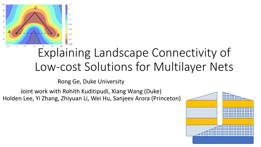
1. Explaining Landscape Connectivity of Low-cost Solutions for Multilayer Nets Rong Ge, Duke University Joint work with Rohith Kuditipudi, Xiang Wang (Duke) Holden Lee, Yi Zhang, Zhiyuan Li, Wei Hu, Sanjeev Arora (Princeton)

2. Mode Connectivity[Freeman and Bruna 16, Garipov et al. 18, Draxler et al. 18] • For neural networks, local minima found via gradient descent are connected by simple paths in the parameter space • Every point on the path is another solution of almost the same cost. Image from [Garipov et al. 18]

3. Outline

4. Background: non-convex optimization • Many objectives are locally optimizable. • Gradient Descent/other algorithms can find a local minimum. • [Jin, G, Netrapalli, Kakade, Jordan 17] Gradient descent finds an -approx local min in iterations. • Many other algorithms known to work [Carmon et al. 2016, Agarwal et al. 2017] All local minima are globally optimal. No high order saddle points. √ x

5. Equivalent local minima and symmetry • Matrix Problems • Goal: find low rank matrix M • Equivalent solutions: • “Tensor” Problems • Goal: find k components • Equivalent solutions: M X XT = (mostly) connected local min Isolated local min Neural networks only have permutation symmetry, why do they have connected local min?

6. (Partial) short answer: overparametrization • Existing explanations of mode connectivity: [Freeman and Bruna, 2016, Venturi et al. 2018, Liang et al. 2018, Nguyen et al. 2018, Nguyen et al. 2019] • If the network has special structure, and is very overparametrized (#neurons > #training samples), then local mins are connected. • Problem: Networks that are not as overparametrized were also found to have connected local min.

7. Our Results • For neural networks, not all local/global min are connected, even in the overparametrized setting. • Solutions that satisfy dropout stability are connected. • Possible to switch dropout stability with noise stability(used for proving generalization bounds for neural nets)

8. Deep Neural Networks • For simplicity: Fully Connected Networks • Weights θ = (W1, W2, …, Wp), nonlinearity σ • Samples (x,y), hope to learn a network that maps x to y • Function • Objective: W1 W3… Wp W2 x(0) = x x(p)= Wpx(p-1) x(1) = σ(W1x) Convex loss function

9. Not all local min are connected • Simple setting: 2-layer net, data (xi, yi) generated by ground truth neural network with 2 hidden neurons. • Overparametrization: consider optimization of a 2 layer neural network with h (h >> 2) hidden neurons. • Theorem: For any h > 2, there exists a data-set with h+2 samples, such that the set of global minimizers are not connected.

10. What kind of local min are connected? • Only local min found by standard optimization algorithms are known to be connected. • Properties of such local min? • Closely connected to the question of generalization/implicit regularization. • Many conjectures: “flat” local min, margin, etc. • This talk: Dropout stability

11. Dropout stability • A network is ε-dropout stable, if zeroing out 50% nodes at every layer (and rescale others appropriately) increases its loss by at most ε. • Theorem: If both θA and θB are ε-dropout stable, then there exists a path between them with maximum loss

12. How to connect a network with its dropout version? High level steps

13. Direct Interpolation • Direct interpolation between the weights does not work. • Even for a simple two layer linear network, if • Interpolation between the parameters with coefficient • In general should have high cost. θA θB

14. Connecting a network with its dropout • Main observation: can use two types of line segments. • Type (a): if θA and θB both have low loss, and they only differ in top layer weight, can linearly interpolate between them. • Type (b): If a group of neurons do not have any outgoing edges, can change their incoming edges arbitrarily. • Idea: Recurse from the top layer, use Type (b) moves to prepare for the next Type (a) move

15. An example path for 3 layer network

16. Example path explained (1) -> (2)

17. Example path explained (2) -> (3)

18. Example path explained (3) -> (4)

19. Example path explained (4) -> (5)

20. Example path explained (5) -> (6)

21. Example path explained (6) -> (7)

22. Noise stability • A network is noise stable, if injecting noise at intermediate layers does not change the output by too much. • Precise definition similar to [Arora et al. 2018] • Theorem: If both θA and θB are ε-noise stable, then there is a path between them with maximum loss . The path consists of 10 line segments. • Idea: noise stability  dropout stability, further, noise stability allow us to do direct interpolation between a network and its dropout.

23. Experiments MNIST, 3-layer CNN CIFAR-10, VGG-11

24. Conclusions

25. Open Problems • Path found by dropout/noise stability are still more complicated than the path found in practice. • Path are known to exist in practice, even if the solutions are not as dropout stable as we hoped. • Can we leverage mode connectivity to design better optimization algorithms?

26. How can we use mode connectivity? • If all local min are connected, then all the level sets are also connected. • If all “typical solutions” are connected (and there is a typical global min), local search algorithms will not be completely stuck. • However, there can still be flat regions/high order saddle points. • Can better optimization/sampling algorithms leverage mode connectivity? Thank you!