Michael A. Nielsen

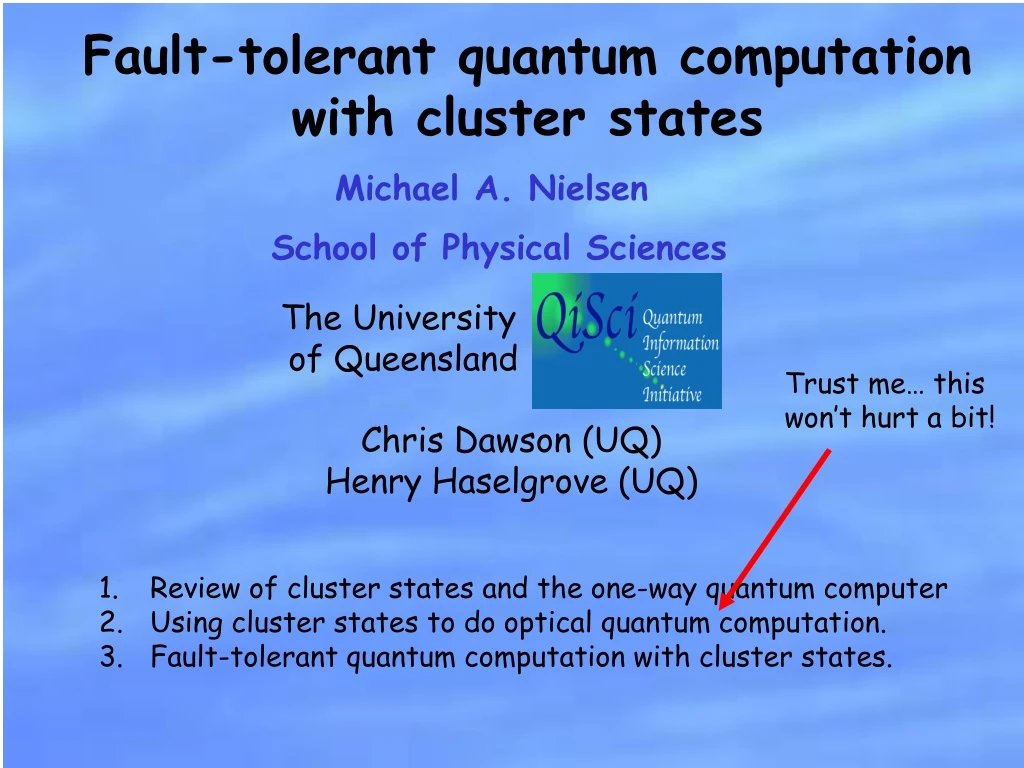
1. Fault-tolerant quantum computation with cluster states Michael A. Nielsen School of Physical Sciences The University of Queensland Trust me… this won’t hurt a bit! Chris Dawson (UQ) Henry Haselgrove (UQ) • Review of cluster states and the one-way quantum computer • 2. Using cluster states to do optical quantum computation. • 3. Fault-tolerant quantum computation with cluster states.

2. Overview of cluster-state computation Three steps: 1. Prepare a many-qubit state, the cluster state. 2. Perform a sequence of adaptive single-qubitmeasurements on some subset of the cluster qubits. 3. The remaining qubits are the output of the computation. These three steps can be used to simulate an arbitrary quantum circuit. (Raussendorf and Briegel, PRL, 2001)

3. Defining the cluster state Each node represents a qubit in the cluster We define the cluster state as the result of the following two-stage preparation procedure. 1. Prepare each qubit in the state |+i´ |0i+|1i 2. Apply a CPHASE gate between each pair of connected qubits. It doesn’t matter in which order the CPHASE gates are applied.

4. Recipe to simulate a quantum circuit The cluster-state simulation Circuit to be simulated |+i HZ2 HZ1 1. HZ1 2. HZ§2 |+i HZ2 HZ1 The gates HZand CPHASE are universal. 1. HZ1 2. HZ§2 U Simulation of an arbitrary circuit follows similar lines. U U

5. What happens if we measure a cluster qubit in the computational basis? Measuring a cluster qubit in the computational basis simply removes it from the cluster.

6. How can we quantum compute with optics? |0i´ horizontally polarized single photon |1i´ vertically polarized single photon Very long decoherence times Operations State preparation Single-qubit gates Measurement Current technology adequate for basic experiments

7. How can we quantum compute with optics? Can we do an entangling gate? CPHASE |xi|yi = (-1)xy |xi |yi Impossible with linear optics alone Knill-Laflamme-Milburn (Nature, 2001) showed how to do this in a non-deterministic but heralded fashion. data Success: A single photon is measured at each port. Occurs with probability ¼. linear optics data Failure: Data measured in the computational basis. ancillas

8. KLM increase the probability of success using two steps. Step 1 Success: A single photon is measured at each port. Occurs with probability (n/(n+1))2. data data linear optics Failure: Data measured in the computational basis. 2n ancillas Making n large increases the success probability, but makes doing the gate harder. We’re going to use n = 2 gate. Succeeds with probability 4/9. We’re actually going to get an effective probability of success 2/3.

9. Step 2 for increasing the probability of success: Probability of success can be boosted closer to 1 using quantum error-correction. Disadvantage: Probability of success close to 1 requires 104-105 optical elements to do a single entangling gate.

10. A better way: combining cluster-state computation with the KLM (2/3)2 gate Suppose we’ve built up part of a cluster… ? And now we attempt to add a qubit. Success: With probability 2/3 we add a qubit to the cluster. Failure: With probability 1/3 we lose a qubit from the cluster. On average, we add 1/3 of a qubit to the cluster, per KLM gate. Of course, it’s not enough just to build up a linear cluster, we need a planar cluster.

11. Building general clusters using the KLM (2/3)2 gate Can build up a general cluster using similar random walk ideas. Result: On average, we add 1/9 th of a qubit to the cluster per KLM gate performed.

12. Summary Basic KLM gate with success probability (2/3)2 can be used to quickly build up clusters. Optical quantum computation (Nielsen, PRL, 2004). Because no error-correction is used, and no value of n greater than 2 is used, more like 102 optical elements are needed for a CPHASE gate – a huge simplification. Claimed experimental demonstration of Rudolph and Browne’s variation, reported by Pan’s group a few days ago. Why this works Failure mode of KLM gate is a computational basis measurement. Coincidentally, such a measurement simply deletes a cluster qubit.

13. What about noise? A proposal for quantum computation should be able to tolerate a reasonable level of physical noise. in abstract circuit models, the techniques of fault-tolerant quantum computation enable a threshold for quantum computation For most proposals (e.g superconductors, KLM, ion trap,…) a physical threshold value follows from straightforward modifications of theoretical threshold constructions. With clusters, fault-tolerance is less obvious. In principle resolution found by Nielsen and Dawson (quant-ph, 2004). C.f. Raussendorf (thesis, 2003), and Aschauer, Durr and Briegel (2004).

14. Basic idea Q: Is it possible to map noise in the CSC back to equivalent noise in the FT circuit? Quantum circuit FT quantum circuit Noisy FT circuit Q: Is “physically reasonable” noise in the CSC mapped back to physically reasonable noise in the FT circuit? ? Cluster- state computation Yes! Such a mapping can be constructed. (Involved.) ? Noisy CSC

15. What properties does the noise mapping have? Local, Markovian noise in CSC Quantum circuit Local, non-Markovian noise of about the same strength. FT quantum circuit Noisy FT circuit Terhal / Burkard (2004): There is a threshold for local non-Markovian noise in quantum circuits. Cluster- state computation There is a threshold for clusters! Noisy CSC

16. Two problems in proving a threshold • If we prepare too much of the cluster at once, some qubitswill decohere. Possible solution … 23. HZ§ Only add extra qubits slowly into the cluster: “just-in-time” preparation. … 23. HZ § 2. If we build the cluster up just-in-time, won’t the stochasticnature of the KLM gate make erasing the cluster a possibility? Yes, but this can be dealt with by building error-correction into the cluster.

17. Preliminary threshold calculations Based on Steane’s approach – our goal at this point is mainly to understand the relationship between circuit and cluster thresholds, not to optimize. We first repeated Steane’s calculations, obtaining: Depolarizing noise y=x No memory noise. Threshold ~ 2E-3 Gate and memory noise equal. x Threshold ~ 5E-4

18. Preliminary threshold calculations We then did a one-buffered cluster simulation, based on Steane’s circuit: Depolarizing noise y=x No memory noise. Threshold ~ 2E-4 Gate and memory noise equal. x Threshold ~ 1E-4

19. Preliminary threshold calculations Improve using parallelizability of Clifford group operations. Improve using purification protocols for cluster states (Aschauer et al). Moving to optical cluster model will also incur additional overhead.

20. Constructing the noise mapping for a toy example 1. HZ1 2. HZ§2 Standard implementation Buffered implementation |+i |+i HZ1 HZ1  HZ1|+i |+i |+i HZ§2 HZ§2 |+i |+i ‘ HZ2HZ1|+i Two points of view: We’ll be interested in both ideal circuit, and the real implementation of the circuit, with noisy elements.

21. Constructing the noise mapping for a toy example (Noisy) buffered cluster state computation |+i HZ1  HZ1|+i |+i HZ§2 |+i ‘ HZ2HZ1|+i Equivalent to:  HZ1|+i |+i ‘ HZ2HZ1|+i |+i HZ1 |+i HZ§2

22. Constructing the noise mapping for a toy example In a more compact form  HZ1|+i ‘ HZ2HZ1|+i |+i |+i |+i HZ§2 HZ1 Insert classical circuitry explicitly.  HZ1|+i |+i ‘ HZ2HZ1|+i |+i |+i HZ§2 HZ§1 0 0

23. Constructing the noise mapping for a toy example With classical circuitry  HZ1|+i ‘ HZ2HZ1|+i |+i |+i |+i HZ§2 HZ§1 0 0 Change classical to quantum  HZ1|+i |+i ‘ HZ2HZ1|+i |+i |+i HZ§2 HZ§1 |0i |0i

24. Constructing the noise mapping for a toy example After changing classical to quantum  HZ1|+i |+i ‘ HZ2HZ1|+i |+i |+i HZ§2 HZ§1 |0i |0i Inserting the identity: HZ1|+i |+i     HZ2HZ1|+i |+i |+i HZ§2 HZ§1 |0i |0i

25. Constructing the noise mapping for a toy example The cluster state computation is made up of repeating blocks of the form: When done perfectly this has the effect: HZ 1   |+i |+i HZ§1 Intuitively, when some of the elements on the left are done imperfectly, we will get a noisy version of the gate on the right.

26. Constructing the noise mapping for a toy example The rigorous connection to the noise model of Terhal and Burkard may be made using the unitary extension theorem. Let U and V be unitaries on T. Inner product space T U and V may have quite different actions on T, but be quite similar on S. Subspace S E.g., |U-V| may be large, while |US – VS| is small. • The unitary extension theorem guarantees the existence of a unitary W • such that • WS = VS • |U - W | · 2 |US – VS| = 2 |US – VS|

27. Constructing the noise mapping for a toy example Can extend the noise mappping to multiple-qubit cluster state computation using similar ideas. The extension to optical cluster-state computation involves similar ideas, but also some additional ideas to cope with the occasional failure of the CPHASE.

28. Constructing the noise mapping: general principles Take the actual (noisy) physical implementation. Imagine it is done noiselessly. Interpret the resulting operations as a (perfect) quantum circuit. Now insert extra elements, which do not change the overall output, but allow us to break the circuit up into blocks, each of which can be interpreted as a gate in the original circuit. The intuition is that when the cluster elements are done noisily, the blocks will function as noisy versions of gates in the original circuit.

29. QIP 2007: QIP-on-the-beach, Queensland