Understanding Data Analysis in Marketing Research: Frequency Distribution and Hypothesis Testing
610 likes | 731 Views
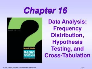
This chapter delves into essential data analysis techniques in marketing research, focusing on frequency distribution, hypothesis testing, and cross-tabulation. It explains how to create frequency distribution tables, interpret key statistics like mean, median, and standard deviation, and emphasizes the steps for hypothesis testing including formulating null and alternative hypotheses. By integrating insights from prior chapters, the chapter presents a cohesive overview that enhances the comprehension of data analysis strategies within the marketing research process, ultimately guiding decision-making.

Understanding Data Analysis in Marketing Research: Frequency Distribution and Hypothesis Testing
E N D
Presentation Transcript
Chapter 16 Data Analysis: Frequency Distribution, Hypothesis Testing, and Cross-Tabulation
Figure 16.1 Relationship of Frequency Distribution, Hypothesis Testing, and Cross-Tabulation to the Previous Chapters and the Marketing Research Process Focus of This Chapter Relationship to Previous Chapters Relationship to Marketing Research Process • Frequency • General Procedure for Hypothesis Testing • Cross Tabulation • Research Questions and Hypothesis (Chapter 2) • Data Analysis Strategy (Chapter 15) Problem Definition Approach to Problem Research Design Field Work Data Preparation and Analysis Report Preparation and Presentation
Fig 16.11 Figure 16.2 Frequency Distribution, Hypothesis Testing, and Cross Tabulation: An Overview Opening Vignette Frequency Distribution Tables 16.1-16.2 Fig 16.3 -16.4 Statistics Associated With Frequency Distribution Fig 16.5 Introduction to Hypothesis Testing What Would You Do? Fig 16.6 -16.9 Be a DM! Be an MR! Experiential Learning Cross Tabulation Tables 16.3-16.5 Statistics Associated With Cross Tabulation Fig 16.10 Cross Tabulation in Practice Fig 16.10 Application to Contemporary Issues (Figs 16.12 – 16.14) International Technology Ethics
Frequency Distribution • In a frequency distribution, one variable is considered at a time. • A frequency distribution for a variable produces a table of frequency counts, percentages, and cumulative percentages for all the values associated with that variable.
Figure 16.3 Conducting Frequency Analysis Calculate the Frequency for Each Value of the Variable Calculate the Percentage and Cumulative Percentage for Each Value, Adjusting for Any Missing Values Plot the Frequency Histogram Calculate the Descriptive Statistics, Measures of Location, and Variability
Table 16.2 Frequency Distribution of Attitude Toward Nike
Table 16.2 (Cont.) Frequency Distribution of Attitude Toward Nike
Statistics Associated with Frequency DistributionMeasures of Location • The mean, or average value, is the most commonly used measure of central tendency. Where, Xi = Observed values of the variable X n = Number of observations (sample size) • The mode is the value that occurs most frequently. It represents the highest peak of the distribution.
Statistics Associated with Frequency DistributionMeasures of Location • The median of a sample is the middle value when the data are arranged in ascending or descending order. If the number of data points is even, the median is usually estimated as the midpoint between the two middle values – by adding the two middle values and dividing their sum by 2. The median is the 50th percentile.
The range measures the spread of the data. It is simply the difference between the largest and smallest values in the sample. Range = - Statistics Associated with Frequency DistributionMeasures of Variability
The variance is the mean squared deviation from the mean. The variance can never be negative. The standard deviation is the square root of the variance. Statistics Associated with Frequency DistributionMeasures of Variability n 2 ( - ) S = n - 1 i = 1
Formulate H0 and H1 Step 1 Step 2 Select Appropriate Test Step 3 Choose Level of Significance, α Step 4 Collect Data and Calculate Test Statistic Determine Probability Associated with Test Statistic (TSCAL) Determine Critical Value of Test Statistic TSCR a) b) Step 5 Compare with Level of Significance, α Determine if TSCAL falls into (Non) Rejection Region a) b) Step 6 Step 7 Reject or Do Not Reject H0 Step 8 Draw Marketing Research Conclusion Figure 16.6 A General Procedure for Hypothesis Testing
A General Procedure for Hypothesis TestingStep 1: Formulate the Hypothesis • A null hypothesis is a statement of the status quo, one of no difference or no effect. If the null hypothesis is not rejected, no changes will be made. • An alternative hypothesis is one in which some difference or effect is expected. Accepting the alternative hypothesis will lead to changes in opinions or actions. • The null hypothesis refers to a specified value of the population parameter (e.g., ), not a sample statistic (e.g., ).
H 1 : p > 0 . 40 A General Procedure for Hypothesis TestingStep 1: Formulate the Hypothesis (Cont.) • A null hypothesis may be rejected, but it can never be accepted based on a single test. In classical hypothesis testing, there is no way to determine whether the null hypothesis is true. • In marketing research, the null hypothesis is formulated in such a way that its rejection leads to the acceptance of the desired conclusion. The alternative hypothesis represents the conclusion for which evidence is sought.
p H H : = 0 . 4 0 1 0 : p ¹ 0 . 4 0 A General Procedure for Hypothesis TestingStep 1: Formulate the Hypothesis (Cont.) • The test of the null hypothesis is a one-tailed test, because the alternative hypothesis is expressed directionally. If that is not the case, then a two-tailed test would be required, and the hypotheses would be expressed as:
A General Procedure for Hypothesis TestingStep 2: Select an Appropriate Test • The test statistic measures how close the sample has come to the null hypothesis and follows a well-known distribution, such as the normal, t, or chi-square. • In our example, the z statistic, which follows the standard normal distribution, would be appropriate. where
A General Procedure for Hypothesis TestingStep 3: Choose a Level of Significance Type I Error • Type Ierror occurs when the sample results lead to the rejection of the null hypothesis when it is in fact true. • The probability of type I error () is also called the level of significance. Type II Error • Type II error occurs when, based on the sample results, the null hypothesis is not rejected when it is in fact false. • The probability of type II error is denoted by . • Unlike , which is specified by the researcher, the magnitude of depends on the actual value of the population parameter (proportion).
A General Procedure for Hypothesis TestingStep 3: Choose a Level of Significance (Cont.) Power of a Test • The power of a test is the probability (1 - ) of rejecting the null hypothesis when it is false and should be rejected. • Although is unknown, it is related to . An extremely low value of (e.g., = 0.001) will result in intolerably high errors. • Therefore, it is necessary to balance the two types of errors.
Figure 16.8 Probability of z With a One-Tailed Test Chosen Confidence Level = 95% Chosen Level of Significance, α=.05 z = 1.645
A General Procedure for Hypothesis TestingStep 4: Collect Data and Calculate Test Statistic In our example, the value of the sample proportion is p= 220/500 = 0.44. The value of can be determined as follows: = = 0.0219
A General Procedure for Hypothesis TestingStep 4: Collect Data and Calculate Test Statistic (Cont.) The test statistic z can be calculated as follows: = 0.44-0.40 0.0219 = 1.83
A General Procedure for Hypothesis TestingStep 5: Determine the Probability (Critical Value) • Using standard normal tables (Table 2 of the Statistical Appendix), the probability of obtaining a z value of 1.83 can be calculated (see Figure 15.5). • The shaded area between - and 1.83 is 0.9664. Therefore, the area to the right of z = 1.83 is 1.0000 - 0.9664 = 0.0336. • Alternatively, the critical value of z, which will give an area to the right side of the critical value of 0.05, is between 1.64 and 1.65 and equals 1.645. • Note, in determining the critical value of the test statistic, the area to the right of the critical value is either or /2. It is for a one-tail test and /2 for a two-tail test.
A General Procedure for Hypothesis TestingSteps 6 & 7: Compare the Probability (Critical Value) and Making the Decision • If the probability associated with the calculated or observed value of the test statistic (TSCAL) is less than the level of significance (), the null hypothesis is rejected. • The probability associated with the calculated or observed value of the test statistic is 0.0336. This is the probability of getting a p value of 0.44 when p= 0.40. This is less than the level of significance of 0.05. Hence, the null hypothesis is rejected. • Alternatively, if the absolute calculated value of the test statistic |(TSCAL)| is greater than the absolute critical value of the test statistic |(TSCR)|, the null hypothesis is rejected.
A General Procedure for Hypothesis TestingSteps 6 & 7: Compare the Probability (Critical Value) and Making the Decision (Cont.) • The calculated value of the test statistic z = 1.83 lies in the rejection region, beyond the value of 1.645. Again, the same conclusion to reject the null hypothesis is reached. • Note that the two ways of testing the null hypothesis are equivalent but mathematically opposite in the direction of comparison. • If the probability of TSCAL < significance level () then reject H0 but if |TSCAL | > |TSCR | then reject H0.
A General Procedure for Hypothesis TestingStep 8: Marketing Research Conclusion • The conclusion reached by hypothesis testing must be expressed in terms of the marketing research problem. • In our example, we conclude that there is evidence that the proportion of customers preferring the new plan is significantly greater than 0.40. Hence, the recommendation would be to introduce the new service plan.
Figure 16.9 A Broad Classification of Hypothesis Testing Procedures Hypothesis Testing Test of Association Test of Difference Means Proportions
Cross-Tabulation • While a frequency distribution describes one variable at a time, a cross-tabulation describes two or more variables simultaneously. • Cross-tabulation results in tables that reflect the joint distribution of two or more variables with a limited number of categories or distinct values, e.g., Table 16.3.
GENDER Female Male Row Total Lights Users14519 Medium Users5510 Heavy Users 51116 Column Total 2421 Table 16.3 A Cross-Tabulation of Gender and Usage of Nike Shoes
Two Variables Cross-Tabulation • Since two variables have been cross classified, percentages could be computed either columnwise, based on column totals (Table 16.4), or rowwise, based on row totals (Table 16.5). • The general rule is to compute the percentages in the direction of the independent variable, across the dependent variable. The correct way of calculating percentages is as shown in Table 16.4.
Table 16.4 Usage of Nike Shoes by Gender
Table 16.5 Gender by Usage of Nike Shoes
Statistics Associated with Cross-TabulationChi-Square • To determine whether a systematic association exists, the probability of obtaining a value of chi-square as large or larger than the one calculated from the cross-tabulation is estimated. • An important characteristic of the chi-square statistic is the number of degrees of freedom (df) associated with it. That is, df = (r - 1) x (c -1). • The null hypothesis (H0) of no association between the two variables will be rejected only when the calculated value of the test statistic is greater than the critical value of the chi-square distribution with the appropriate degrees of freedom, as shown in Figure 16.10.
Figure 16.10 Chi-Square Test of Association Figure 16.10 Chi-Square Test of Association Level of Significance, α 2
Statistics Associated with Cross-TabulationChi-Square The chi-square statistic (2)is used to test the statistical significance of the observed association in a cross-tabulation. The expected frequency for each cell can be calculated by using a simple formula: where = total number in the row = total number in the column = total sample size
Expected Frequency For the data in Table 16.3, for the six cells from left to right and top to bottom = (24 x 19)/45 = 10.1 = (21 x 19)/45 =8.9 = (24 x 10)/45 = 5.3 = (21 x 10)/45 =4.7 = (24 x 16)/45 = 8.5 = (21 x 16)/45 =7.5
= (14 -10.1)2 + (5 – 8.9)2 10.1 8.9 + (5 – 5.3)2 + (5 – 4.7)2 5.3 4.7 + (5 – 8.5)2 + (11 – 7.5)2 8.5 7.5 = 1.51 + 1.71 + 0.02 + 0.02 + 1.44 + 1.63 = 6.33
Statistics Associated with Cross-TabulationChi-Square • The chi-square distribution is a skewed distribution whose shape depends solely on the number of degrees of freedom. As the number of degrees of freedom increases, the chi-square distribution becomes more symmetrical. • Table 3 in the Statistical Appendix contains upper-tail areas of the chi-square distribution for different degrees of freedom. For 2 degrees of freedom, the probability of exceeding a chi-square value of 5.991 is 0.05. • For the cross-tabulation given in Table 16.3, there are (3-1) x (2-1) = 2 degrees of freedom. The calculated chi-square statistic had a value of 6.333. Since this is greater than the critical value of 5.991, the null hypothesis of no association is rejected indicating that the association is statistically significant at the 0.05 level.
Statistics Associated with Cross-TabulationPhi Coefficient • The phi coefficient () is used as a measure of the strength of association in the special case of a table with two rows and two columns (a 2 x 2 table). • The phi coefficient is proportional to the square root of the chi-square statistic: • It takes the value of 0 when there is no association, which would be indicated by a chi-square value of 0 as well. When the variables are perfectly associated, phi assumes the value of 1 and all the observations fall just on the main or minor diagonal.
Statistics Associated with Cross-TabulationContingency Coefficient • While the phi coefficient is specific to a 2 x 2 table, the contingency coefficient(C) can be used to assess the strength of association in a table of any size. • The contingency coefficient varies between 0 and 1. • The maximum value of the contingency coefficient depends on the size of the table (number of rows and number of columns). For this reason, it should be used only to compare tables of the same size.
Statistics Associated with Cross-TabulationCramer’s V • Cramer's V is a modified version of the phi correlation coefficient, , and is used in tables larger than 2 x 2. or
Cross-Tabulation in Practice While conducting cross-tabulation analysis in practice, it is useful to proceed along the following steps: * Test the null hypothesis that there is no association between the variables using the chi-square statistic. If you fail to reject the null hypothesis, then there is no relationship. * If H0 is rejected, then determine the strength of the association using an appropriate statistic (phi-coefficient, contingency coefficient, or Cramer's V), as discussed earlier. * If H0 is rejected, interpret the pattern of the relationship by computing the percentages in the direction of the independent variable, across the dependent variable. Draw marketing conclusions.
Figure 16.11 Conducting Cross-Tabulation Analysis Construct the Cross-Tabulation Data Calculate the Chi-Square Statistic, Test the Null Hypothesis of No Association Reject H0? NO YES No Association Determine the Strength of Association Using an Appropriate Statistic Interpret the Pattern of Relationship by Calculating Percentages in the Direction of the Independent Variable
SPSS Windows: Frequencies • The main program in SPSS is FREQUENCIES. It produces a table of frequency counts, percentages, and cumulative percentages for the values of each variable. It gives all of the associated statistics. • If the data are interval scaled and only the summary statistics are desired, the DESCRIPTIVES procedure can be used. • The EXPLORE procedure produces summary statistics and graphical displays, either for all of the cases or separately for groups of cases. Mean, median, variance, standard deviation, minimum, maximum, and range are some of the statistics that can be calculated.
SPSS Windows: Frequencies To select these frequencies procedures, click the following: • Analyze > Descriptive Statistics > Frequencies . . . • Or Analyze > Descriptive Statistics > Descriptives . . . • or Analyze > Descriptive Statistics > Explore . . . We illustrate the detailed steps using the data of Table 16.1.