Download
1 / 18
180 likes | 358 Views
SFitter: Determining SUSY Parameters. R é mi Lafaye, Tilman Plehn, Michael Rauch, Dirk Zerwas. What do we do? (1). From a set of measurements: Low scale indirect constraints M top , BR(b s ), (g-2) , M W , sin 2 eff , BR(B s + - ) Or dark matter constraints h 2 from WMAP

E N D
SFitter: Determining SUSY Parameters Rémi Lafaye, Tilman Plehn, Michael Rauch, Dirk Zerwas
What do we do? (1) • From a set of measurements: • Low scale indirect constraints • Mtop, BR(bs), (g-2), MW, sin2eff, BR(Bs+-) • Or dark matter constraints h2 from WMAP • LHC measurements (di-lepton edges, sqR 10mass difference, …) • Or ATLAS+CMS measurements (no need to be combined) • And then ILC measurements • Compare to Susy theoretical predictions: • Spectrum calculators: • Suspect [A. Djouadi, J.L. Kneur & G. Moultaka] • Softsusy [B.C. Allanach] • Isasusy [H. Baer, F.E. Paige, S.D. Protopopescu & X. Tata] • LHC Cross sections: Prospino2 [T. Plehn et al.] • LC Cross sections: MsmLib [G. Ganis] • Branching ratios: Hdecay, Sdecay[A. Djouadi, M. Mühlleitner & M. Spira] • Dark matter: Micromegas[G. Bélanger, F. Boudjema, A. Pukhov & A. Semenov] R. Lafaye - Wednesday, 27 June 2007
What do we do ? (2) Then, find best 2 using different fitting technics: • Minuit, Grid scan • Markov chains (to be described here) Measurements defined as: x:= ( xexp exp syst and xth th ) Where: • exp is gaussian and might be correlated • systis gaussian and 99% correlated (LHC jet or lepton energy scale) • thtwo possibilities (see next slides) Needs careful likelihood (L) study to extract parameter errors: • 2 = -2 ln(L) • Best method is to smear input values according to uncertainties • And perform a set of toy-experiments • Start with a two constraints toy-model fit R. Lafaye - Wednesday, 27 June 2007
Theoretical errors (1) Lmax First case: Treat theoretical errors as gaussian • Bayesian: assumes a pdf for theoretical predictions • Correlation between experimental uncertainties is smeared out • The gaussian tails extend far away from the usually admitted theoretical range xexp-xth yexp-yth L xexp-xth R. Lafaye - Wednesday, 27 June 2007
Theoretical errors (2) Lmax Second case: Use Rfit scheme [A.Hoecker, H.Lacker, S.Laplace, F.Lediberder] if(|xexp-xth|< th) 2 = 0 else 2 = [(|xexp-xth|-th)/exp]2 xexp-xth There is no convolution between experimental and theoretical errors Just a theoretically allowed range for xth yexp-yth L xexp-xth R. Lafaye - Wednesday, 27 June 2007
Markov Chains (1) Definition: The future state depends on the current but not on the past Principle: • Starts from a point in the parameter space. Compute 2cur • Pick a new point (using Monte-Carlo technics) and compute 2new • Switch to new point • if 2new <2cur • or Random[0,1] < 2cur /2new Advantages: • Faster than crude scan, for N parameters: cN c1 N (instead of c1N) • Markov chains do not rely on 2 shape in parameter space (no use of gradients) • Ability to find secondary minima ( to a grid scan) Drawbacks: • Exact minimum not found (use gradient fit around minima to improve) • Choice of new point implies the use of priors (like for any Monte-Carlo) • Bad choice of priors Limited parameter space region scanned R. Lafaye - Wednesday, 27 June 2007
Markov Chains (2) Choosing the next point: • Flat: Pick parameter values evenly between the allowed range • Breit-Wigner: Has higher tails than gaussian, can go to zero at bounds • Using BW can speed up the convergence if the 2 gradients are “nice” Choosing the “right” priors: Problem: for a parameter “x” should we use a prior as a function of x, 1/x, ln(x) ? Any choice will bias the fit toward a given parameter space region Theoretically increasing the number of points in the chains can overcome this Or alternatively, one can try different priors and make sure the whole parameter space is correctly scanned Note that this last problem is not specific to Markov Chains as long as the 2 distribution has secondary minima. At least Markov Chains offer a solution. R. Lafaye - Wednesday, 27 June 2007
mSUGRA at LHC mSUGRA SPS1a as a benchmark point: m0=100 GeV, m1/2=250 GeV, tan=10, A0=-100 GeV, >0 and mtop=171.4 GeV The LHC “experimental” data from cascade decays: ~ ~ q q 02 02 l lR lR l 02 ~ ~ ~ ~ Theoretical errors: • 3% for gluino and squark masses • 1% for other sparticle masses R. Lafaye - Wednesday, 27 June 2007
mSUGRA Markov Chains Scan SPS1a benchmark point results from Markov Chains • SFitter output #1: fully inclusive likelihood map • SFitter output #2: ranked list of local maxima m1/2 z axis: minimum 2 found in all other directions (tan, A0, , mtop) m0 R. Lafaye - Wednesday, 27 June 2007
Markov Chains priors 2 different priors for tan: • Right: Flat prior (use the low scale parameter tan) • Left: Use the high scale parameter B 1/ tan2 Number of points • Around tan=10 the two priors picks an equivalent number of points • Choosing the B prior favors low values of tan 1/2min R. Lafaye - Wednesday, 27 June 2007
Frequentist or Bayesian (1) SFitter provide a multi-dimensional likelihood map One can then perform his favorite analysis… Bottom: Frequentists look for lower 2 in all other directions Top: Bayesians marginalize the 2 in all other directions B prior tan prior 1/2marg • Choice of the prior has a lot of influence on the marginalized plots • 2min shape remains the same. But the true minimum might not be found More points or use Minuit around minima 1/2min R. Lafaye - Wednesday, 27 June 2007
Frequentist or Bayesian (2) Left: flat (Rfit) theoretical errors Right: gaussian errors m1/2 2min mtop m0 m0 2min R. Lafaye - Wednesday, 27 June 2007 A0 A0
Frequentist or Bayesian (3) Left: Frequentist: 2min and flat (Rfit) theoretical errors Right: Bayesian: marginalize 2 and gaussian errors, B prior m1/2 • Bayesian preferred solutions: • m0 = 50 GeV • m1/2 = 250 GeV • A0 = 1400 GeV • mtop = 169 GeV mtop m0 m0 2 R. Lafaye - Wednesday, 27 June 2007 A0 A0
mSUGRA Markov Chains SPS1a benchmark point results from Markov Chains • SFitter output #1: fully inclusive likelihood map • SFitter output #2: ranked list of local maxima sgn() m1/2 R. Lafaye - Wednesday, 27 June 2007
mSUGRA Minuit Results Perform a Minuit fit around the best minimum 2 point: No correlations, no theoretical errors, Sign(μ) fixed • To be done: • Include correlations and theoretical errors • Proper CL coverage using Rfit scheme (non gaussian case) • Define 2 p-value: mSUGRA & measurements agreement • using Monte-Carlo toys R. Lafaye - Wednesday, 27 June 2007
pMSSM Fit mSUGRA: 6D parameter space [including sgn()] pMSSM: 15D parameter space Use of Markov Chains makes a scan possible Lack of sensitivity on one parameter does not slow down the scan (no need to use fixed parameters) Low sensitivity on tan R. Lafaye - Wednesday, 27 June 2007
pMSSM up to GUT Scale Testing unification [SFitter+J.L. Kneur] Still need to include low scale parameter errors for completness R. Lafaye - Wednesday, 27 June 2007
Summary SFitter combines measurements from different sources into a determination of supersymmetric parameters • Markov Chains: • Speed up the scan of the parameter space • Especially useful for large number of parameters • Provide likelihood map and ranked list of minima • Frequentist or Bayesian: • Both can be performed from the likelihood map • Bayesian output greatly depends on the choice of priors • Full frequentist analysis needs a lot of “toys” • Work in progress: • Minuit fit around minima including all uncertainties • Full frequentist treatment including 2min p-value and coverage determination R. Lafaye - Wednesday, 27 June 2007