
Segmentation
E N D
Presentation Transcript
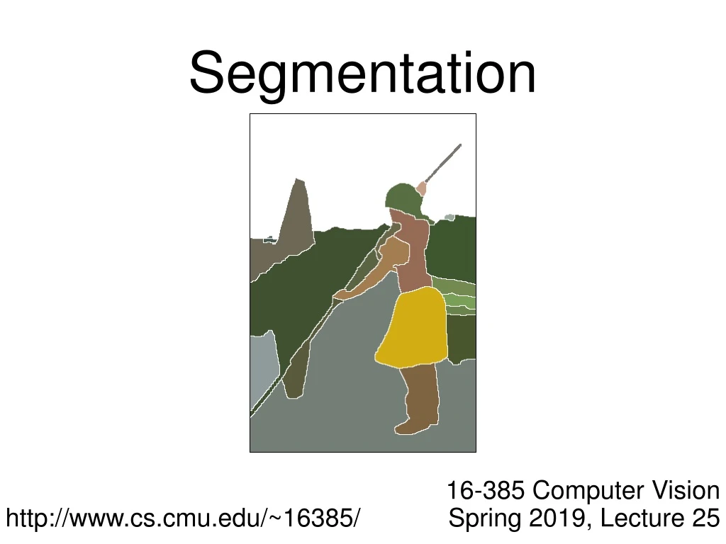
Segmentation 16-385 Computer Vision Spring 2019, Lecture 25 http://www.cs.cmu.edu/~16385/
Overview of today’s lecture Finish temporal models. Normalized cuts. Boundaries. Clustering for segmentation.
Slide credits Most of these slides were adapted from: Srinivasa Narasimhan (16-385, Spring 2015). James Hays (Brown University).
Image segmentation by pairwise similarities • Image = { pixels } • Segmentation = partition of image into segments • Similarity between pixelsiandj • Sij = Sji≥ 0 Sij • Objective: “similar pixels, with large value of Sij, should be in the same segment, dissimilar pixels should be in different segments” Computer Vision
Relational Graphs • G=(V, E, S) • V: each node denotes a pixel • E: each edge denotes a pixel-pixel relationship • S: each edge weight measures pairwise similarity • Segmentation = node partitioning • break V into disjoint sets V1, V2 Computer Vision
i Sij j A i A B Weighted graph partitioning Pixels iI = vertices of graph G Edges ij = pixel pairs with Sij > 0 Similarity matrixS = [ Sij ] di = Sj Є GSij degree of I deg A = Si Є A di degree of A G Assoc(A,B) = Si Є ASj Є B Sij Computer Vision
Cuts in a Graph • (edge) cut = set of edges whose removal makes a graph disconnected • weight of a cut: cut( A, B ) = Si Є A, Sj Є B Sij =Assoc(A,B) • the normalized cut • Normalized Cut criteria: minimum cut(A,Ā) NCut( A,B ) = cut(A, B)( + ) 1 deg A 1 deg B Computer Vision
Grouping with Spectral Graph Partitioning SGP: data structure = a weighted graph, weights describing data affinity Segmentation is to find a node partitioning of a relational graph, with minimum total cut-off affinity. Discriminative models are used to evaluate the weights between nodes. The solution sought is the cuts of the minimum energy. NP-Hard! Computer Vision
Matrix representation of the graph problem: 5 0.1 4 1 6 2 3 4 2 3 9 7 2 5 1 7 2 1 1 8 2 0.1 2 affinity matrix
Eigenvector approach to segmentation Represent a connected component (or clusterC) By aweight vector w such that (indicator vector): wtMw is the association of C because: • If C is a good cluster, then the average association between features • In C should be large. Therefore, we want: • wtMw is large • Suggests algorithm: • Build matrix M • Find w such that wtMw is maximum. • Problem: w is a binary vector
Replace binary vector with continuous weight vector. Interpretation: • wi large if i belongs to C. • Problem becomes: • Find w such that wtMw is maximum • Construct the corresponding component C by: • i belongs to C if wi is large. • Problem with scale: • The relative values of the wi’s are important, the total magnitude of w is not. • Normalization:
Replace binary vector with continuous weight vector. Interpretation: • wi large if i belongs to C. • Problem becomes: • Find w such that wtMw is maximum • Construct the corresponding component C by: • i belongs to C if wi is large. • Problem with scale: • The relative values of the wi’s are important, the total magnitude of w is not. • Normalization: Rayleigh’s ratio theorem: Given a symmetric matrix M, the maximum of the ratio is obtained for the eigenvector wmax corresponding to the largest eigenvalue lmax of M.
Brightness Image Segmentation Computer Vision
Brightness Image Segmentation Computer Vision
Results on color segmentation Computer Vision
Prob. of boundary • Intuition: • Duality between regions and boundaries • Maybe “easier” to estimate boundaries first • Then use the boundaries to generate segmentations at different levels of granularity • All examples from: P. Arbelaez, M. Maire, C. Fowlkes and J. Malik. Contour Detection and Hierarchical Image Segmentation. IEEE TPAMI, Vol. 33, No. 5, pp. 898-916, May 2011. • Complete package: http://www.eecs.berkeley.edu/Research/Projects/CS/vision/grouping/resources.html Fine resolution Coarse resolution
Brightness Color 1 Combining multiple cues Color 2 Texton
gPb (global Pb) • Idea: We could use the Pb contours to generate an affinity matrix and then use Ncuts • j and i have lower affinity because they cross higher Pb values
gPb (global Pb) Good: Combine the gradients of the eigenvectors!! Not good: generate segmentation from the eigenvectors
Final step: Convert closed boundary (UCM = Ultrametric Contour Map) • Different thresholds on contours yield segmentations at different levels of granularity • Guaranteed to produce a hierarchical segmentation
Prob. of boundary • Intuition: • Duality between regions and boundaries • Maybe “easier” to estimate boundaries first • Then use the boundaries to generate segmentations at different levels of granularity • Complete package: http://www.eecs.berkeley.edu/Research/Projects/CS/vision/grouping/resources.html Fine resolution Coarse resolution
Clustering: group together similar points and represent them with a single token Key Challenges: 1) What makes two points/images/patches similar? 2) How do we compute an overall grouping from pairwise similarities?
Why do we cluster? • Summarizing data • Look at large amounts of data • Patch-based compression or denoising • Represent a large continuous vector with the cluster number • Counting • Histograms of texture, color, SIFT vectors • Segmentation • Separate the image into different regions • Prediction • Images in the same cluster may have the same labels
How do we cluster? • K-means • Iteratively re-assign points to the nearest cluster center • Agglomerative clustering • Start with each point as its own cluster and iteratively merge the closest clusters • Mean-shift clustering • Estimate modes of pdf
2. Assign each object to the cluster with the nearest centroid. 1. Select initial centroids at random
2. Assign each object to the cluster with the nearest centroid. 1. Select initial centroids at random 3. Compute each centroid as the mean of the objects assigned to it (go to 2)
2. Assign each object to the cluster with the nearest centroid. 1. Select initial centroids at random 3. Compute each centroid as the mean of the objects assigned to it (go to 2) 2. Assign each object to the cluster with the nearest centroid.
2. Assign each object to the cluster with the nearest centroid. 1. Select initial centroids at random 3. Compute each centroid as the mean of the objects assigned to it (go to 2) 2. Assign each object to the cluster with the nearest centroid. Repeat previous 2 steps until no change
K-means Clustering Given k: • Select initial centroids at random. • Assign each object to the cluster with the nearest centroid. • Compute each centroid as the mean of the objects assigned to it. • Repeat previous 2 steps until no change.
K-means: design choices • Initialization • Randomly select K points as initial cluster center • Or greedily choose K points to minimize residual • Distance measures • Traditionally Euclidean, could be others • Optimization • Will converge to a local minimum • May want to perform multiple restarts
K-means clustering using intensity or color Image Clusters on intensity Clusters on color
How to choose the number of clusters? • Minimum Description Length (MDL) principal for model comparison • Minimize Schwarz Criterion • also called Bayes Information Criteria (BIC)
K-Means pros and cons • Pros • Finds cluster centers that minimize conditional variance (good representation of data) • Simple and fast* • Easy to implement • Cons • Need to choose K • Sensitive to outliers • Prone to local minima • All clusters have the same parameters (e.g., distance measure is non-adaptive) • *Can be slow: each iteration is O(KNd) for N d-dimensional points • Usage • Rarely used for pixel segmentation
Agglomerative clustering How to define cluster similarity? • Average distance between points, maximum distance, minimum distance • Distance between means or medoids How many clusters? • Clustering creates a dendrogram (a tree) • Threshold based on max number of clusters or based on distance between merges distance
Conclusions: Agglomerative Clustering Good • Simple to implement, widespread application • Clusters have adaptive shapes • Provides a hierarchy of clusters Bad • May have imbalanced clusters • Still have to choose number of clusters or threshold • Need to use an “ultrametric” to get a meaningful hierarchy
Mean shift segmentation D. Comaniciu and P. Meer, Mean Shift: A Robust Approach toward Feature Space Analysis, PAMI 2002. • Versatile technique for clustering-based segmentation
Mean shift algorithm • Try to find modes of this non-parametric density
Mean Shift Algorithm A ‘mode seeking’ algorithm Fukunaga & Hostetler (1975)
Mean Shift Algorithm A ‘mode seeking’ algorithm Fukunaga & Hostetler (1975) Find the region of highest density