Segmentation
Explore various segmentation methods including region-based, watershed, and graph-based approaches for separating objects from backgrounds in images. Learn about region growing, splitting, and merging techniques for effective segmentation results.

Segmentation
E N D
Presentation Transcript
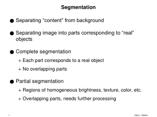
Segmentation • Separating “content” from background • Separating image into parts corresponding to “real” objects • Complete segmentation • Each part corresponds to a real object • No overlapping parts • Partial segmentation • Regions of homogeneous brightness, texture, color, etc. • Overlapping parts, needs further processing
Segmentation Methods • Based on global knowledge • Thresholding based on histogram • Edge-based • Region-based • Combinations of the last two • Edge-based and region-based are duals of each other
Region Based Segmentation • Goal: find regions that are “homogeneous” by some criterion • Region Growing • Start with tiny regions, combine neighboring regions that are sufficiently similar to each other • Need: initialization, similarity criterion • Region Splitting • Start with one big region, separate regions that are not sufficiently homogeneous • Need: homogeneity criterion, split rule
Region Growing Example (Haralick & Shapiro) • Assume: region is connected component with the same population mean and variance • Initialization: R is a single pixel (e.g. top-left) • Similarity Criterion: region R to neighboring pixel y • Compute the mean intensity value of R • Compute the scatter (variance) of R • Compute a T-value (H&S 10.14) - measures difference between y and the "typical pixel" in R • If T is small enough, add y to R and recompute statistics • Otherwise, y cannot be added to R -- either find another compatible neighboring region, or start a new one
Region Growing (Watershed) • Smooth the image • Run an edge detector (get gradient magnitude = edge strength) • Create a ‘seed’ at each local min i.e. where there is no edge. • Essentially, the idea is to ‘flood’ the image, marking each pixel as it goes ‘underwater’
Watershed Example val = 0 While (unmarked pixels exist){ for(pixel in image) if (pixel.val = val) if 2 neighbors are different pixel is border else if no neighbors are marked pixel is seed else mark pixel = neighbor val++ }
Improving Watershed • Instead of using all minima, user selects minima directly. • “pixel is seed” test removed from algorithm • Use morphology to clean up local boundaries, smooth edges (e.g. closing) Figure 5.14
Region Splitting Example (Ohlander) • Push a mask consisting of the entire image • While the stack is not empty • Pop a mask from the stack • Compute Histogram of the current mask • Divide the histogram into clusters (find valleys between peaks) • If there are multiple peaks • For each peak, compute connected components and push a mask for each • Else, label all pixels in mask as one region • Result: Set of regions in the image (each a connected component)
Interpreting the example • Homogeneity criterion • Single-peak histogram • Split rule • Split according to histogram peak/valley analysis • Consider separate connected components as separate regions
Growing and Splitting • Combining splitting and merging may yield best regions • Better than splitting alone, because splitting is constrained to specific “split” boundaries • Better than merging alone, because merging two whole regions might be overkill • Use hierarchical data structure: split moves down, merge moves up
Graph Based Segmentation • Image graph: • Each vertex is a region • Each edge is a boundary between two regions • Each edge has a weight corresponding to the dis-similarity between regions (e.g. intensity difference)
Graph Based Segmentation (Cont) • Initialize the graph as one region per pixel • For each region R, internal difference = largest edge weight in minimum spanning tree [ Int(R)] • Difference between R1 and R2 is minimum edge weight connecting the two regions (i.e. any pixel from R1 to any pixel from R2) [Diff(R1, R2)] • If Diff(R1,R2) < min(Int(R1)+p(R1), Int(R2)+p(R2)) merge R1 and R2 • p(R) is a region penalty they set to k / (region area) • Merge regions in decreasing order of the edges separating them, i.e. most dissimilar first
Quadtree • Data structure that captures multiple scales • Tree structure, where each tree represents a square subimage. • Each subimage can have 4 children (upper-left quadrant, upper-right, lower-left, and lower-right) • If region is homogeneous, it is a leaf (no matter how big) • Smallest regions are single pixels (and they are always leaves)
Split & Merge with Quadtrees • Initialize segmentation (arbitrarily or using prior knowledge) • For each region R, if it is not homogeneous, split it. This builds a quadtree. • If R1 and R2 are neighbors, and they can be merged into a homogeneous region, do it. (This might destroy the quadtree structure, because you might get a 1/4 region connected to a 1/16 region) • If any regions are “too small”, merge them with the “best” neighbor.
K-means Segmentation • Goal: threshold a multi-dimensional histogram to find clusters • In theory, 5-dimensional histogram (3 color + 2 location) • In reality, just pick 2 or 3 dimensions (e.g. L*a*b*)
Displaying & Representing Regions • Overlays (for display) • Use bright colors to show regions over greytone image • Color border pixels to contrast (e.g. white, red) • Labeled image • Each region has a unique identifier (e.g. integer) • In a copy of the image, set each pixel value to its region label • For display, use well-separated values (grey or color)