Elementary Probability Theory
Elementary Probability Theory. Chapter 5 of the textbook Pages 145-164. Introduction. Statistical Decision Theory – using the probability of possible outcomes to choose between several available options Statistical Inference – using samples to infer the probabilities of the population.

Elementary Probability Theory
E N D
Presentation Transcript
Elementary Probability Theory Chapter 5 of the textbook Pages 145-164
Introduction • Statistical Decision Theory – using the probability of possible outcomes to choose between several available options • Statistical Inference – using samples to infer the probabilities of the population
Definitions • Statistical Experiment • Measuring an elementary outcome that is not known in advance • Elementary Outcome • Each possible outcome of a statistical experiment • If the experiment was to test gender in this classroom the elementary outcomes would be male and female • Sample Space • The set of all possible elementary outcomes
Sample Space Examples • Definition: the set of all possible outcomes of an experiment. • Examples of sample spaces: • Outcomes of the roll of a die: {1, 2, 3, 4, 5, 6} • Outcomes of 2 coin flips: {HH, HT, TH, TT} • Outcomes of rolling 2 dice:
Definitions • Events • Subsets of the sample space • Each event contains 1 or more elementary outcomes • Event Space • All the elementary outcomes that constitute an event • Complimentary Event • All elementary outcomes not in the event space
Event • An outcome or a set of outcomes • Examples of events: • Roll of one die: {2} • Roll of one die: {2, 5} • Roll of two dice: {2 and 4}, {4 and 3} • Roll of two dice: {1 and 2, 5 and 6} • Flip coin once: {H} • Flip coin twice: {HT}
Example • Assume I sampled a people on the bus and asked their ages and got the following results • 19, 20, 20, 23, 27, 31, 37, 42, 56, 58 • How many elementary outcomes do I have? • If I break the sample space into events by decade (e.g., 20s) what are my events? • What is the event space of each event? • What is the complimentary event of the 50s event?
Symbols • P() – The probability of something (usually an outcome or an event) • Ei – An elementary outcome, note the “i” which ranges from 1 to n • (S) – The sample space (you may also see (Ω)) • A, B, … – Events are typically assigned to capital letters • – Complimentary events are the event letter with a bar • Ø – Null (i.e., no solution)
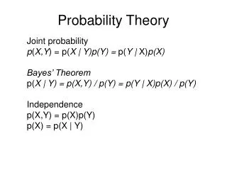
Relationships Between Events • Remember – each experiment has 1 and only 1 elementary outcome, but an outcome can be in 1 or more events • Intersection: the event space that is shared (i.e., the outcome is in both (or all) event spaces) • Example: overlapping portion of the Venn Diagram • Union: combination of event spaces, (i.e., the outcome is in at least 1 event)
A B UNION A INTERSECTION B Venn Diagrams
Probability Postulates • P(Ei) probability of an outcome is between 0 and 1 (0 = impossible, 1 = certain) • P(A) = = sum of probabilities of all elementary outcomes in the event space • P(S) = 1 = certain • P(Ø) = 0 = impossible
Rules Derived From Postulates • The sum of all elementary outcomes is 1 (certain) • The probability of an event is between 1 and zero** • If A and B are mutually exclusive P(A ∩ B) = Ø ** Note the book incorrectly uses “≤” in this rule
Types of Probability • Subjective: an event probability with accuracy/validity based on the experience of and information available to an observer • Objective: an event probability determined by the frequency of elementary outcomes observed during statistical experimentation
Calculating Probability • When all outcomes are equally likely, the probability of an event A: • m = the number of elementary outcomes in the event space • n = the number of elementary outcomes in the sample space • In other words…. • P(A) = Total number of ways to achieve the event Total number all possible outcomes
Calculating Probability Example • Experiment: coin toss • P(heads) = 1 / 2 = 0.5 • The number of elements in the event space (m) = 1 (i.e., heads) • The number of elements in the sample space (n) = 2 (i.e., heads or tails) • Experiment: roll a die. • P(rolling a 6) = 1 / 6 = 0.166667 • The number of elements in the event space (m) = 1 (i.e., a 6) • The number of elements in the sample space (n) = 6 (i.e., 1,2,3,4,5,or 6)
Complicating Factors • What do we do when all outcomes are not equally likely? • Answer: “the subset of the sample space that comprises the event space must be specified… the [sum] of the elementary outcome probabilities in the event space will yield the event probability” • Conceptually this just means that we back up a step and calculate the probability of the outcomes and add them up for each event (think frequency tables)
A Familiar Example • Assume I sampled a people on the bus and asked their ages and got the following results: • 19, 20, 20, 23, 27, 31, 37, 42, 56, 58 • What is the probability of getting a result of 31? • P(answer of 31) = 1 / 10 = 0.1 • What is the probability of getting a result in the 30s? • P(30s) = P(answer of 31) + P(answer of 37) = 0.1 + 0.1 = 0.2 • What is the probability of getting a result in the 20s? • P(20s) = P(answer of 20) + P(answer of 23) + P(answer of 27) = 0.2 + 0.1 +0.1 = 0.4
Counting Rules • These are some useful rules for determining the elementary outcome counts (which are used to determine probabilities) • These are useful for many applications beyond just calculating probability • Symbol Confusion • The book uses “r” in two different ways • For the product rule each “r” is a group and each group has n elements (i.e., r1 has n1 elements, r2 has n2 elements…) • For the combinations and permutations rules each “r” is a subset of a larger group and “r” indicates the size (i.e. the number of elements) in the group being formed
Product Rule • Used to calculate all possible combinations available when selecting one member from each available group • Number of possible combinations = n1 * n2 …. • Example: Flipping a coin 3 times • Each flip is a group and each flip has 2 possible outcomes (n1 = n2 = n3 =2) • The number of possible outcomes is 2*2*2 = 8 • Outcomes = {HHH}, {HHT}, {HTH}, {HTT}, {THH}, {THT}, {TTH}, {TTT}
Combinations Rule • Used to select all the possible groups of size r from the sample space • Since the sample space has n outcomes, r ≤ n • Example: • 4 cards - A, K, Q, J • How many combinations can you have if you pick 2 cards (r=2) • AK, AQ, AJ, KQ, KJ, QJ
Permutations Rule • Used to select all the possible groups of size r from the sample space including the order of the elements • Since the sample space has n outcomes, r ≤ n • Example: • 4 cards - A, K, Q, J • How many combinations can you have if you pick 2 cards (r=2) • AK, AQ, AJ, KQ, KJ, QJ • KA, QA, JA, QK, JK, JQ
Hypergeometric Rule • The combination of the product rule and the combination rule • Since the sample space has n outcomes, r ≤ n • Example: • 2 sets of 4 cards (A, K, Q, J) and (1, 2, 3, 4) • How many combinations can you have if you pick 2 cards (r=2) from each set? • Answer = 36
A B UNION Probability Theorems • Addition Theorem • Rule of thumb: Union uses addition
Examples • Coin Flip: • P(heads) = 0.5 • P(tails) = 0.5 • P(heads ∩ tails) = 0 • Cards • P(heart) = 13/52 • P(king) = 4/52 • P(heart ∩ king) = 1/52
Probability Theorems • Complementation Theorem • Recall that P(S) = 1
Probability Theorems • Conditional Probability • Think of this as the probability of X given Y where both X and Y have their own probability • Intuition should tell you that this will hinge on the intersection of X and Y
Probability Theorems • Statistically Independent Events – the probability of an event remains the same despite the occurrence of another event • Example: The probability of a coin flip being heads is ½ regardless of what the last coin flip was • Based on conditional probability
A INTERSECTION B Probability Theorems • Multiplication Theorem • Rule of thumb: Intersections use multiplication
Statistically Independent Examples • 2 Coin Flips • A and B are the probability of getting heads • P(heads) = 1/2 • P(heads ∩heads) = P(A|B) * P(B) = ¼ • P(heads | heads on first flip) = P(heads ∩heads) / P(B) = (¼) / (½) = 1/2 • Draw 2 cards • P(heart) = 13/52 • P(king) = 4/52 • P(heart ∩ king) = 1/52 • P(heart | king) = P(heart ∩ king) / P(king) = (1/52) / (4/52) = 13/52 = 1/4 • P(king | heart) = P(heart ∩ king) / P(heart) = (1/52) / (13/52) = 4/52 = 1/13
Statistically Dependent Example • Probability of drawing 2 hearts • Drawing single cards from a complete deck would equate to: • P(A) = P(heart) = 13/52 • P(B) = P(heart) = 13/52 • P(A|B) = P(heart|heart on last draw) = 12/51 • Solution 1: imagine drawing 1 card and then the second: • (A ∩ B) = P(A|B) * P(B) = 0.589 • Solution 2: imagine drawing both cards at once • Remember P(event) = m/n • n = number of all combinations (full sample space) • m = number of possible combinations of 2 hearts (event space) • Both m and n are calculated using the combinations rule • m = n = • P(drawing 2 hearts) = 78/1326 = 0.589