Download
1 / 36
360 likes | 381 Views
Turbulent Transport in Single-Phase Flow Peter Bernard, University of Maryland. Assume that our goal is to compute mean flow statistics such as. and. where. One can either: Pursue DNS (i.e. the "honest" approach) of averaging solutions of the NS eqn:.

E N D
Turbulent Transport in Single-Phase Flow Peter Bernard, University of Maryland
Assume that our goal is to compute mean flow statistics such as and where One can either: Pursue DNS (i.e. the "honest" approach) of averaging solutions of the NS eqn: or pursue RANS (i.e. the "dishonest" approach) of solving the averaged NS eqn: where the Reynolds stress tensor, is modeled.
DNS: Highly accurate but of limited practical usefulness. RANS: Inaccurate, unreliable, requires empirical modeling, but of widespread use. LES, a third approach has conceptual problems - though these are usually ignored. In particular, the average of the filtered velocity: does not necessarily equal the mean velocity, i.e. Moreover, if where is the resolved part of the velocity fluctuation, then Conundrum: if the subgrid energy is large, then K cannot be found. If the subgrid energy is small, then LES is a DNS.
Our interest here is in the RANS approach. There are 2 basic options: Direct models for or model the equation: Direct models are most popular and we consider just this case.
The Reynolds stress Rij has a physical interpretation as the flux of the ith component of momenum in the jth direction caused by the fluctuating velocity field. For non-dense gases the stress tensor in the Navier-Stokes equation has a similar interpretation as representing the flux of the ith component of momentum in the jth direction due to molecular motion. In the molecular case: and the stress tensor is:
Can a similar model for the Reynolds stress tensor be justified?
There are very strong reasons for wanting such a model to be true. In this case the mean momentum equation becomes: • This approach is: • easy to install within a NS solver • relatively well behaved • relatively inexpensive to solve
Consider the validity of the molecular transport analogy in the context of a turbulent transport in a unidirectional mean flow such as in a channel or boundary layer: In this case:
U(y) l Molecules transport momentum, unchanged, over the mean free path, l, before colliding with other molecules and exchanging momentum. U(y) is linear over l. here:
To analyze the physical mechanisms behind turbulent transport consider the set of fluid elements that arrive at a given point a at time t. t t-t b local linear approximation a b b b • Unlike the molecular case: • momentum is not preserved on paths until mixing. • the idea of "mixing" is undefined • no obvious separation of scales
Use backward particle paths to evaluate an exact Lagrangian decomposition of the Reynolds shear stress that exposes the underlying physics. goes to 0 as t increases (establishes a mixing time). Thus transport caused by fluid particles carrying, unchanged, the mean momentum at point b to point a. transport associated with changes in velocity (accelerations) along particle paths.
The correlation is created by fluid particle movements within a spatially varying mean field: when v > 0 the difference in mean velocity along the path is negative and vice versa.
Acceleration transport originates largely in the effect of vortical structures in accelerating fluid particles as they move toward the wall (sweeps) or retarding fluid particles as they eject from near the wall. Close to the surface, viscous effects retard fast moving fluid particles leading to a decrease in Reynolds stress.
Decomposition of acceleration transport into viscous and pressure effects.
Evaluation of the Lagrangian decomposition in channel flow yields: transport due to particle accelerations transport due to particle displacements
The Lagrangian analysis can yield a quantitative estimate of the potential errors in a gradient model of the Reynolds stress. (Mixing length - distance traveled during the mixing time) effect of non-linearity of the mean velocity over the mixing length gradient term
An exact decomposition of the turbulent shear stress: Correct gradient Non-linearity Acceleration contribution of mean velocity effects where Lagrangian integral time scale
Errors in the gradient model: Clearly , significant errors are present. RANS models attempt to compensate for errors by a judicious choice of the eddy viscosity.
Dissatisfaction with linear transport models has fueled interest in models that are non-linear in: (rotation tensor) (rate of strain tensor) A typical example of a non-linear model (e.g. Algebraic RS Models): Sometimes non-linear models are derived by simplification of RSE models.
Assuming some legitimacy for linear RS models - what is nt ? For molecular transport: suggesting that the eddy viscosity depends on the product of velocity (U) and length (L) scales. RANS models vary depending on the choice for U and L. The K - e closure assumes (eddy turnover time) Thus:
K equation modeling Production From e equation sK is a turbulent Prandtl number
e equation Production Transport/Diffusion Dissipation
Modeling of the e equation is done in stages by considering its properties in simplified settings: 1. isotropic decay. 2. homogeneous shear flow. 3. constant stress layer near solid walls.
The exact equations governing the decay of Isotropic Turbulence: vortex stretching dissipation After defining: (skewness) (palenstrophy) Reynolds number These may be simplified to:
In the case of self-similarity, e.g.: SK and G are constant and the system of equations is closed and solvable. Two equilibria exist: Low RT : vortex stretching negligible: High RT : vortex stretching and dissipation equilibrate In traditional modeling vortex stretching is eliminated creating an opportunity to match decay rate with experiments:
Homogeneous shear flow is constant everywhere exact equations Assume: enstrophy
Modeled Equations for Homogeneous Shear Flow Without vortex stretching: blow up. With vortex stretching: prod = diss equilibrium chosen to match experiments
e equation modeling homogeneous shear flow model - calibrated to give correct K growth Isotropic turbulence model - calibrated to give a decay rate consistent with data
Calibration of the K-e Closure In the "constant stress layer" Assume: and the model: Then: Moreover, if then: Substituting these results into the e equation gives:
Near-wall modeling Boundary conditions: Among the problems with the high Re modeling near a boundary: Introduce a wall function to force the equivalence: In effect,
Other problems that have to be fixed near a wall: K → 0 at wall so dissipation blows up At the wall surface: yet no explicit model for Pe has been assumed in high Re model.
Low Re model for the e equation near walls. wall functions here (e.g.)
What to expect from the popular RANS models: 1. The predictions of RANS models in their standard form, can be both acceptable or unacceptable depending on the desired accuracy, naivety of the user and other factors. 2. It is very common to make ad hoc changes to the values of constants and even to add additional modeling expressions in order to improve accuracy, or to force the solution to acquire desired physical attributes. The idea is that some aspect of physics is lacking in the original model that needs to be compensated for. 3. Changing the properties of models can bring the solutions closer to one set of data and further from another set of data. 4. Sometimes model alterations - with no basis in physics - are made as a last resort to force better results: e.g. "clipping" 5. RANS solutions sometimes are regarded as successful if only one part of the solution is captured - the part that is of interest.
6. Adding additional physics to RANS calculations can be especially difficult - two layers of inaccuracy: the underlying turbulence and the new physical model. Different models of the physics (e.g. particle dispersion, chemistry, combustion) can react differently to the same underlying RANS modeling. 7. A numerical calculation with a RANS scheme may converge for one set of input parameters and not converge for a similar case of the same flow. 8. The quality of one particular RANS model may appear to be better than it is because if performs better than other models. 9. Very often computational speed is considered more important than accuracy. 10. In some flows, complaints about steady RANS solutions have led to the use of URANS (Unsteady RANS) in which features such as vortex shedding are considered to be part of the mean (albeit transient) field.
11. Many research studies have compared LES predictions to RANS predictions. Sometimes RANS is as good as LES, sometimes LES is better, sometimes the added accuracy of LES is not justified by the cost. 12. RANS is increasingly being used to model the wall region of LES since the local DNS resolution that one would hope for is often not feasible.