Turbulent flow models
Turbulent flow models. Katarzyna Miłkowska - Piszczek. Faculty of Metal Engineering and Industrial Computer Science Department of Ferrous Metallurgy Kraków 8.12.2010. Content. Preface CFD Turbulence models DNS LES K/ ε. Turbulent flow. I n fluid dynamics , turbulence or

Turbulent flow models
E N D
Presentation Transcript
Turbulent flow models Katarzyna Miłkowska - Piszczek Faculty of Metal Engineering and Industrial Computer Science Department of Ferrous Metallurgy Kraków 8.12.2010
Content • Preface • CFD • Turbulence models • DNS • LES • K/ε
Turbulent flow In fluid dynamics , turbulence or turbulent flow is a fluid regime characterized by chaotic, stochastic property changes. This includeslow momentum diffusion ,high momentum convection and rapidvariation of pressure and velocity in space andtime.
Turbulent flow • The fundamental mathematical model are the non-isothermal Navier-Stokesequations, governing the time-evolution of velocity, pressure and temperature. • The phenomenon of turbulence reveals that their solutions can become very complex if a critical parametere.g., the Reynolds number or the Rayleigh number, becomes large
Preface A proper numerical resolution of the random motion of allscales of ~u, ~p, and ~ T (called DirectNumericalSimulation)is feasible only for a very limitednumber of flows. Thus the major task in turbulencemodeling is to reducethe complexity of the Navier-Stokes equations in a mannerwhich is appropriate to the needs of science andengineering. The goal is to develop models that arecomputationallysimpler than the Navier-Stokes equationsbut "whose predictions are closeto those of the Navier-Stokes equations".
Preface • The first approach is a statistical approach which is based on a statistical averaging procedure forthe Navier-Stokes equations. The objective is to obtain a set of equations for the statisticalmean values for ~u, ~p, and ~ T, which requires an empirical modelling of the terms involving statistical fluctuations. • The second approach is called large-eddy simulation (LES). Theidea of LES is to apply a spatial averaging filter to the Navier-Stokes equations in order toextract the large-scale structures of ~u, ~p, and ~ T, and to attenuate their small-scale structures. Then only the random motion of the large scales is resolved and the effects of thesmall scales on the large scales are modelled.
Preface Then the turbulent state of motion is simply the phenomenological aspect of this complexity.The complexity of the solution has two aspects, viz., its randomness its vast and continuous range of scalesthe turbulence problem is how to describe and how to reduce this complexity in a manner which is appropriate to the needs of science and engineering.
Preface • compute the random motion of all scales,which is referred to as direct numerical simulation (abbreviated DNS) • compute the random motion of the largescale motion (and model the small scalemotion), which is referred to as large-eddy simulation (abbreviatedLES) • predict mean flow field, pressure andtemperature (in astatistical sense), referred toas statisticalturbulence modelling orReynolds averagedCFD (called RANS)
Classes of turbulence models • RANS-basedmodels • Lineareddy-viscositymodels • Algebraicmodels • One and twoequationmodels • Non-lineareddyviscositymodels and algebraicstressmodels • Reynolds stress transport models • Largeeddysimulations • Detachededdysimulations and otherhybridmodels • Directnumericalsimulations
CFD Computational fluid dynamics (CFD) is a branch of fluid mechanics that uses numerical method and algorithms to solve and analyze problems that involve fluid flows. Computers are used to perform the calculations required to simulate the interaction of liquids and gases with surfaces defined by boundary conditions. With high-speed supercomputers, better solutions can be achieved. Ongoing research, however, yield software that improves the accuracy and speed of complex simulation scenarios such as transonic or turbulent flows.
The Kolmogorov scale A direct numerical simulation (DNS) is a simulation in computational fluid dynamics in which theNavier-Stokes equations are numerically solved without any turbulence model. This means that the whole range of spatial and temporal scales of the turbulence must be resolved. All the spatial scales of the turbulence must be resolved in the computational mesh, from the smallest dissipative scales ( Kolomogorov scales) , up to the integral scale L, associated with the motions containing most of the kinetic energy. The Kolmogorov scale is given by: where ν is the kinematic viscosity , ε is the rate of kinetic energy dissipation.
Dissipation of turbulent kinetic energy By a production mechanism Pthe large eddies are generated. These are unstable and break up into successively smaller and smaller eddies, i.e. theirenergy is transferred to smaller and smaller scales byinviscid processes. At the smallestscales the energy is dissipated into heat by molecular viscosity. This process is calleddissipation of turbulent kinetic energyor simply dissipation.
The Kolmogorov thesis Kolomogorov postulated that for very high Re the small scale turbulent motions are statistically isotropic (i.e. no preferential spatial direction could be discerned). In general, the large scales of a flow are not isotropic, since they are determined by the particular geometrical features of the boundaries (the size characterizing the large scales will be denoted as L).
The Kolmogorov thesis A turbulent flow is characterized by a hierarchy of scales through which the energy cascade takes place. Dissipation of kinetic energy takes place at scales of the order of Kolmogorov length η, while the input of energy into the cascade comes from the decay of the large scales, of order L. These two scales at the extremes of the cascade can differ by several orders of magnitude at high Reynolds numbers. In between there is a range of scales (each one with its own characteristic length r) that has formed at the expense of the energy of the large ones.
The Kolmogorov thesis Since eddies in this range are much larger than the dissipative eddies that exist at Kolmogorov scales, kinetic energy is essentially not dissipated in this range, and it is merely transferred to smaller scales until viscous effects become important as the order of the Kolmogorov scale is approached. Within this range inertial effects are still much larger than viscous effects, and it is possible to assume that viscosity does not play a role in their internal dynamics (for this reason this range is called "inertial range").
The Kolmogorov thesis At very high Reynolds number the statistics of scales in the range η≤ r ≤ L are universally and uniquely determined by the scale r and the rate of energy dissipation .
DNS The integral scale depends usually on the spatial scale of the boundary conditions. To satisfy these resolution requirements, the number N of points along a given mesh directionwith increments h, must be : N h > L so that the integral scale is contained within the computational domain, and also h ≤ ηso that the Kolmogorov scale can be resolved. Since ε≈u' ³ / L where u' is the root mean square (RMS) of the velocity
DNS The previous relations imply that a three-dimensional DNS requires a number of mesh points satisfying N³ where Re is the turbulent Reynolds number the memory storage requirement in a DNS grows very fast with the Reynolds number. In addition, given the very large memory necessary, the integration of the solution in time must be done by an explicit method.
DNS C is here the Courant number : Combining these relations, and the fact that h must be of the order of , the number of time-integration steps must be proportional to L / C η. By other hand, from the definitions for Re, η and L given above, it follows that and consequently, the number of time steps grows also as a power law of the Reynolds number
DNS One can estimate that the number of floating-point operations required to complete the simulation is proportional to the number of mesh points and the number of time steps, and in conclusion, the number of operations grows as Re³ . Therefore, the computational cost of DNS is very high,even at low Re. For the Reynolds numbers encountered in most industrial applications, the computational resources required by a DNS would exceed the capacity of the most powerful computer currently available.
DNS Also, direct numerical simulations are useful in the development of turbulence models for practical applications, such as sub-grid scale models for LESand models for methods that solve the Reynolds- averaged Navier-Stokes equations (RANS). This is done by means of "a priori" tests, in which the input data for the model is taken from a DNS simulation, or by "a posteriori" tests, in which the results produced by the model are compared with those obtained by DNS.
Property of turbulent flow A major property of turbulent flows is that they appear to be chaotic or random. Randomnessis a consequenceof the interaction of • the singular perturbation parameter Re resp. Raand • the non-linearity of the Navier-Stokes equations In a fluid flow experiment, thereare unavoidably inaccuracies and perturbations in initial conditions, boundary conditions (e.g., differential heating, surface roughness) and material properties, i.e. viscosity andthermal diffusivity (due to impurities of the fluid).
The scales of turbulent flow A second characteristic feature of a turbulent flow is its large variety of scales. Understanding of the different scales of motion in turbulent flows andthe processes among them, being a motivation for the approach of large-eddy simulation (LED). Turbulent flow can be thought of as a superposition of locally coherent structures, called eddies, of different sizes. Today, the term 'eddy' is used moreambiguously; it is used to characterise the scales of structures in the flow field: Largeeddies refer to large structures, small eddies refer to small structures in the flow field
LES Large eddy simulation is a mathematical model for turbulence used in computational fluid dynamic. LES grew rapidly and is currently applied in a wide variety of engineering applications, including combustion, acoustics, and simulations of the atmospheric boundary layer.
Type of LES models • Smagorinsky-Lilly model • Dynamic subgrid-scale model • RNG-LES model • Wall-adapting local eddy-viscosity (WALE) model • Kinetic energy subgrid-scale model • Near-wall treatment for LES models
K/ε model The k/ε model is the most widespread turbulence model, but it suffers from severalwell-known deficiencies. A successful improvement of the standard k/ ε model is the so called k-ε -υ² model. This model requires resolving the near-wall region,which is infeasible for three-dimensional problems of practical relevance.
K/ε model The model solves the turbulent closure problem by adding two transport equations to the Reynolds-averaged Navier-Stokes equations: • one for the turbulent kinetic energyk [m² / s²] • one for the rate of turbulent dissipation ε [m² / s³] A turbulent velocity scale is then given by: υ = √ k [ m /s] and a turbulent time scale asГ = k/ ε [s]
K/ε model For the case of an incompressible flow, thetransport equations are given by where the production term P is
K/ε model The turbulent kinematic viscosity is then modeled as : The standard constans values of the model :
K/ε model The coeffcients are determined by demanding that this turbulence model should satisfy experimental datafor certain simple standard flow cases. coeffcient is obtained by considering the log-law region of a turbulentboundary layer. The is usually fixed from calibrations with homogeneous shear flows, and is usually determined from the decay rate ofhomogeneous, isotropic turbulence. , are optimized by applying the modelto various fundamental flows such as flow in channel, pipes, jets, wakes.
K/ε model Because the standard K/ε model is derived under the assumption of a high (local) turbulent Reynoldsnumber, regions of low turbulent Reynolds number, such as close to the wall, are poorly modeled. In thoseregions the destruction-of-dissipation term is singular at the wall since ε is finite and the turbulent kinetic energy k is zero.
K/ε model Two-equation turbulence modelswidely used in industrial CFD applications although their shortcomings are well known. The model coefficients in turbulence modeling are usually kept constant in turbulentflows with different geometry and at different Reynolds numbers. The use of these asymptotic constraints on the model constants provides a formally-consistent model. The k-ε model constants have assumed different values depending on the applications.
RANS based turbulence models • Lineareddyviscositymodels • Twoequationmodels • k-epsilonmodels • Standard k-epsilon model • Realisablek-epsilon model • RNG k-epsilon model • Near-walltreatment • k-omegamodels • Wilcox'sk-omega model • Wilcox'smodifiedk-omega model • SST k-omega model • Near-walltreatment
Reference list • R.W .Lewis. , K. Ravindran and A.S. Usmani, „Finite Element Solution of Incompressible FlowsUsing an Explicit Segregated Approach”, Archives of Computational Methods in Engineering, Vol. 2, 4, 69–93 (1995). • A.T. Patera, „ A spectral element method for fluid dynamics: Laminar flow in a channel expansion”, Journal of Computationing Physics 54, 468-488 (1984). • R.Peyret, T.D. Taylor, „Computational Methods for Fluid Flow”, Springer-Verlag New York Inc., 1983, USA. • O.C. Zienkiewicz, „The finite element method” Fourth Edition Volume 1 Basic Formulation and Linear Problems, McGraw-Hill International (UK), 1989, Londyn. • O.C. Zienkiewicz, „The finite element method” Fourth Edition Volume 2 Solid and Fluid Mechanics Dynamics and Non-linearity, McGraw-Hill International (UK), 1991, Londyn.