
Mastering Data Preprocessing for Effective Analysis
E N D
Presentation Transcript
Outline • Why preprocess the data? (為何要做資料的預處理) • Descriptive data summarization (資料的摘要性描述) • Data cleaning (資料清理) • Data integration and transformation (資料整合與轉換) • Data reduction (資料縮減) • Discretization and concept hierarchy generation (離散化與概念分層的產生) • Summary
Why Data Preprocessing? • Data in the real world is dirty–只要人一多,什麼樣的怪腳都可能會出現!! • Incomplete (不完整的): • lacking attribute values, lacking certain attributes of interest • e.g., occupation=“” • Noisy (含噪音的): • containing errors or outliers • e.g., Salary=“-10” • Inconsistent (不一致的): • containing discrepancies in codes or names • e.g., Age=“42” Birthday=“03/07/1997” • e.g., Was rating “1,2,3”, now rating “A, B, C” • e.g., discrepancy between duplicate records
Why Is Data Dirty? • Incomplete data may come from • “Not applicable (不合用)” data value when collected • Different considerations between the time when the data was collected and when it is analyzed. • Human/hardware/software problems • Noisy data (incorrect values) may come from • Faulty data collection instruments (如: 問卷設計不良) • Human or computer error at data entry • Errors in data transmission • Inconsistent data may come from • Different data sources • Functional dependency (功能相依性) violation (e.g., modify some linked data)
Why Is Data Preprocessing Important? • No quality data, no quality mining results! • Quality decisions must be based on quality data • e.g., duplicate or missing data may cause incorrect or even misleading statistics. • Data warehouse needs consistent integration of quality data • Data extraction, cleaning, and transformation comprises the majority of the work of building a data warehouse
Multi-Dimensional Measure of Data Quality • A well-accepted multidimensional view: • Accuracy (精確性) • Completeness (完整性) • Consistency (一致性) • Timeliness (及時性) • Believability (可信度) • Value added (附加價值) • Interpretability (可解釋性) • Accessibility (易接受)
Major Tasks in Data Preprocessing • Data cleaning (資料清理) • Fill in missing values, smooth noisy data, identify or remove outliers, and resolve inconsistencies • Data integration (資料整合) • Integration of multiple databases, data cubes, or files • Data transformation (資料轉換) • Normalization and aggregation • Data reduction (資料縮減) • Obtains reduced representation in volume but produces the same or similar analytical results • Data discretization (資料離散化) • Part of data reduction but with particular importance, especially for numerical data
Data Cleaning • Data cleaning tasks • Fill in missing values (填寫空缺值) • Identify outliers and smooth out noisy data (識別孤立點與消除噪音資料) • Correct inconsistent data (解決不一致資料)
Missing Data • Data is not always available • E.g., many tuples have no recorded value for several attributes, such as customer income in sales data • Missing data may be due to • equipment malfunction (設備異常) • inconsistent with other recorded data and thus deleted (與其它已存在資料不一致而遭刪除) • data not entered due to misunderstanding (因為誤解而資料沒有被輸入) • certain data may not be considered important at the time of entry (在輸入時,因為得不到應用的重視而沒有被輸入) • Missing data may need to be inferred.
How to Handle Missing Data? • Ignore the tuple: • usually done when class label is missing (assuming the tasks in classification—not effective when the percentage of missing values per attribute varies considerably. • Fill in the missing value manually: • tedious + infeasible? • Fill in it automatically with • a global constant : • e.g., “unknown” • a new class?! • the attribute mean • the attribute mean for all samples belonging to the same class: smarter • the most probable value: • inference-based such as Bayesian formula or decision tree
Noisy Data • Noise: random error or variance in a measured variable • Incorrect attribute values may due to • faulty data collection instruments (資料收集工具的缺失) • data entry problems (資料輸入問題) • data transmission problems (資料傳輸問題) • technology limitation (技術限制) • inconsistency in naming convention (命名規則不一致) • Other data problems which requires data cleaning • duplicate records (重覆記錄) • incomplete data (不完整的資料) • inconsistent data (不一致的資料)
How to Handle Noisy Data? • Binning (分箱) • first sort data and partition into (equal-depth) bins • then one can smooth by bin means, smooth by bin median, smooth by bin boundaries, etc. • Regression (回歸) • smooth by fitting the data into regression functions • Clustering (聚類) • detect and remove outliers • Combined computer and human inspection (電腦與人工判斷的結合) • detect suspicious values by computer, and check by human (e.g., deal with possible outliers)
Simple Discretization Methods: Binning • Binning methods smooth a stored data value by consulting its “neighborhood” (the values around it). • Equal-width (distance) partitioning • Divides the range into N intervals of equal size • e.g., Box 1: 1 ~ 10, Box 2: 11 ~ 20, Box 3: 21 ~ 30, … • Equal-depth (frequency) partitioning • Divides the range into N intervals, each containing approximately same number of samples • e.g., 每一個Box都可以存放4筆資料
Binning Methods for Data Smoothing • Step 1: * Sorted data for price (in dollars): 4, 8, 9, 15, 21, 21, 24, 25, 26, 28, 29, 34 * Partition into equal-depth bins: - Bin 1: 4, 8, 9, 15 - Bin 2: 21, 21, 24, 25 - Bin 3: 26, 28, 29, 34 • Step 2: * Smoothing by bin means: - Bin 1: 9, 9, 9, 9 - Bin 2: 23, 23, 23, 23 - Bin 3: 29, 29, 29, 29 * Smoothing by bin boundaries: - Bin 1: 4, 4, 4, 15 - Bin 2: 21, 21, 25, 25 - Bin 3: 26, 26, 26, 34
y Y1 y = x + 1 Y1’ x X1 Regression
Data Integration • Data integration: • Combines data from multiple sources into a coherent store • There are a number of issues to consider during data integration. • Schema integration (概要整合) • Redundancy (冗餘資料) • Detection and resolution of data value conflicts (資料值衝突的偵測與解決) • Careful integration of the data from multiple sources may help reduce/avoid redundancies and inconsistencies and improve mining speed and quality
Schema integration: • Identify real world entities from multiple data sources • Entity identification problem: • e.g., A.cust-id B.cust-# • Integrate metadata from different sources • Metadata最常見的英文定義是〝data about data 〞,可直譯為描述資料的資料,主要是描述資料屬性的資訊 • Examples of metadata for each attribute include the name, meaning, data type, and rang of values permitted for the attribute. • Can be used to help avoid errors in schema integration. • Detecting and resolving data value conflicts: • For the same real world entity, attribute values from different sources are different • Possible reasons: • different representations, • different scales, • e.g., metric (公制) vs. British (英制) units
Handling Redundancy in Data Integration • Redundant data occur often when integration of multiple databases, because: • The same attribute or object may have different names in different databases • One attribute may be a “derived” attribute in another table, e.g., annual revenue • Redundant attributes may be able to be detected by correlation analysis
Correlation Analysis (Numerical Data) • Correlation coefficient (also called Pearson’s product moment coefficient) where n is the number of tuples, and are the respective means of A and B, σA and σB are the respective standard deviation of A and B, and Σ(AB) is the sum of the AB cross-product. • If rA,B > 0, A and B are positively correlated (A’s values increase as B’s). The higher, the stronger correlation. • rA,B = 0: independent; rA,B < 0: negatively correlated
Correlation Analysis (Categorical Data 類別資料) • Χ2 (chi-square) test • The larger the Χ2 value, the more likely the variables are related • The cells that contribute the most to the Χ2 value are those whose actual count is very different from the expected count • Correlation does not imply causality • # of hospitals and # of car-theft in a city are correlated • Both are causally linked to the third variable: population
Chi-Square Calculation: An Example • Χ2 (chi-square) calculation (numbers in parenthesis are expected counts calculated based on the data distribution in the two categories) • It shows that like_science_fiction and play_chess are correlated in the group
Data Transformation • Smoothing (平滑): remove noise from data • Aggregation (聚集): summarization, data cube construction • Generalization (一般化): concept hierarchy climbing • Normalization (正規化): scaled to fall within a small, specified range • min-max normalization • z-score normalization • normalization by decimal scaling • Attribute construction (屬性構造): • New attributes constructed from the given ones
Data Transformation: Normalization • Min-max normalization: to [new_minA, new_maxA] • Ex. Let income range $12,000 to $98,000 normalized to [0.0, 1.0]. Then $73,000 is mapped to • Z-score normalization (μ: mean, σ: standard deviation): • Ex. Let μ = 54,000, σ = 16,000. Then • Normalization by decimal scaling Where j is the smallest integer such that Max(|ν’|) < 1
Data Reduction Strategies • Why data reduction? (為何需要資料縮減?) • A database/data warehouse may store terabytes of data • Complex data analysis/mining may take a very long time to run on the complete data set • Data reduction • Obtain a reduced representation of the data set that is much smaller in volume but yet produce the same (or almost the same) analytical results • Data reduction strategies • Data cube aggregation (資料立方體聚集) –aggregation operations • Attribute subset selection (屬性子集合選擇) - e.g.,remove unimportant attributes • Dimensionality reduction (維度縮減), Data Compressed (資料壓縮) –encoding mechanism • Numerosity reduction (數值縮減) - e.g.,fit data into models • Discretization and concept hierarchy generation (離散化和概念分層產生)
Data Cube Aggregation • Data cubes store multidimensional aggregated information. • Data cubes are discussed in detail in Chapter 3 • For example:
Attribute Subset Selection • Data sets for analysis may in hundreds of attributes, many of which may be irrelevant to the mining task or redundant. • Reduce the data set size by removing irrelevant or redundant attributes (or dimensions). • The goal of attribute subset selection is to find a minimum set of attributes such that the resulting probability distribution of the data classes is as close as possible to the original distribution obtained using all attributes.
How can we find a ‘good’ subset of the original attributes? • For n attributes, there are 2n possible subsets. • Heuristic methods (due to exponential # of choices): • Step-wise forward selection (向前逐步選擇) • Step-wise backward elimination (向後逐步排除) • Combining forward selection and backward elimination (結合向前逐步選擇與向後逐步排除) • Decision-tree induction (決策樹歸納)
Original Data Compressed Data lossless lossy Original Data Approximated Dimensionality Reduction • Data encoding or transformations are applied so as to obtain a reduced or “compressed” representation of the original data. • Lossless (無損壓縮): If the original data can be reconstructed from the compressed data without any loss of information. • Lossy (有損壓縮): we can reconstruct only an approximation of the original data.
String compression (字串壓縮) • There are extensive theories and well-tuned algorithms • Typically lossless • But only limited manipulation is possible without expansion • Audio/video compression • Typically lossy compression, with progressive refinement • Sometimes small fragments of signal can be reconstructed without reconstructing the whole • Two popular and effective methods of lossy dimensionality reduction: • Wavelet transforms (微波轉換) • Principal components analysis (主成份分析)
Numerosity Reduction • Reduce data volume by choosing alternative, smaller forms of data representation • Parametric methods • Assume the data fits some model, estimate model parameters, store only the parameters, and discard the data (except possible outliers) • Example: Log-linear models—obtain value at a point in m-D space as the product on appropriate marginal subspaces • Non-parametric methods • Do not assume models • Major families: histograms, clustering, sampling
Regress Analysis and Log-Linear Models • Linear regression: Y = w X + b • Two regression coefficients, w and b, specify the line and are to be estimated by using the data at hand • Using the least squares criterion to the known values of Y1, Y2, …, X1, X2, …. • Multiple regression: Y = b0 + b1 X1 + b2 X2. • Many nonlinear functions can be transformed into the above • Log-linear models: • The multi-way table of joint probabilities is approximated by a product of lower-order tables • Probability: p(a, b, c, d) = ab acad bcd
Histograms • Divide data into buckets and store average (sum) for each bucket • Partitioning rules: • Equal-width • Equal-frequency (or equal-depth)
Clustering • Partition data set into clusters based on similarity, and store cluster representation (e.g., centroid and diameter) only • Can be very effective if data is clustered, but not if data is “smeared” (資料界限模糊) • Can have hierarchical clustering and be stored in multi-dimensional index tree structures • There are many choices of clustering definitions and clustering algorithms • Cluster analysis will be studied in depth in Chapter 7
Sampling • Sampling: obtaining a small sample s to represent the whole data set N • The most common ways: • Simple random sample without replacement (SRSWOR) of size s • Draw a tuple, record it, and not replaced • The probability of drawing any tuple in D is 1/N • Simple random sample with replacement (SRSWR) of size s • Draw a tuple, record it, and replaced • A tuple may be draw again • Cluster sample • Grouped the tuples in D into M mutually disjoint clusters • An SRS of s clusters can be obtained. • Stratified sample • D is divided into mutually disjoint parts called strata • A stratified sample of D is generated by obtaining an SRS at each stratum.
Raw Data Sampling: with or without Replacement SRSWOR (simple random sample without replacement) SRSWR
Sampling: Cluster or Stratified Sampling Cluster/Stratified Sample Raw Data
Discretization • Three types of attributes: • Nominal— values from an unordered set, e.g., color, profession • Ordinal— values from an ordered set, e.g., military or academic rank • Continuous —numbers, e.g., integer or real numbers • Discretization: • Divide the range of a continuous attribute into intervals • Some classification algorithms only accept categorical attributes. • Reduce data size by discretization • Prepare for further analysis
Discretization and Concept Hierarchy • Discretization • Reduce the number of values for a given continuous attribute by dividing the range of the attribute into intervals • Interval labels can then be used to replace actual data values • Discretization can be performed recursively on an attribute • Concept hierarchy formation • Recursively reduce the data bycollecting and replacing low level concepts (such as numeric values for age) by higher level concepts (such as young, middle-aged, or senior)
Discretization and Concept Hierarchy Generation for Numeric Data • Typical methods: All the methods can be applied recursively • Binning (covered above) • Top-down split, unsupervised, • Histogram analysis (covered above) • Top-down split, unsupervised • Clustering analysis (covered above) • Either top-down split or bottom-up merge, unsupervised • Entropy-based discretization: supervised, top-down split • Segmentation by natural partitioning: top-down split, unsupervised
Entropy-Based Discretization • Given a set of samples S, if S is partitioned into two intervals S1 and S2 using boundary T, the information gain after partitioning is • Entropy is calculated based on class distribution of the samples in the set. Given m classes, the entropy of S1 is where pi is the probability of class i in S1 • The boundary that minimizes the entropy function over all possible boundaries is selected as a binary discretization • The process is recursively applied to partitions obtained until some stopping criterion is met • Such a boundary may reduce data size and improve classification accuracy
Segmentation by Natural Partitioning • 聚類分析產生概念分層可能會將一個工資區間劃分為︰[51263.98, 60872.34] • 通常數據分析人員希望看到劃分的形式為[50000,60000] • A simply 3-4-5 rule can be used to segment numeric data into relatively uniform, “natural” intervals.
Steps: • 如果一個區間最高有效位上包含3,6,7或9個不同的值,就將該區間劃分為3個等寬子區間;(72,3,2) • 如果一個區間最高有效位上包含2,4,或8個不同的值,就將該區間劃分為4個等寬子區間; • 如果一個區間最高有效位上包含1,5,或10個不同的值,就將該區間劃分為5個等寬子區間; • 將該規則遞迴的應用於每個子區間,產生給定數值屬性的概念分層; • 對于數據集中出現的最大值和最小值的極端分佈,為了避免上述方法出現的結果扭曲,可以在頂層分段時,選用一個大部分的機率空間。e.g. 5%-95%
Concept Hierarchy Generation for Categorical Data • 分類資料是指無序的離散資料,它有有限個值(可能很多個) • 分類資料的概念分層之生成方法: • Specification of a partial/total ordering of attributes explicitly at the schema level by users or experts • street < city < state < country • Specification of a hierarchy for a set of values by explicit data grouping • {Urbana, Champaign, Chicago} < Illinois • Specification of only a partial set of attributes • E.g., only street < city, not others • Automatic generation of hierarchies (or attribute levels) by the analysis of the number of distinct values • E.g., for a set of attributes: {street, city, state, country}
15 distinct values country 365 distinct values province_or_ state 3567 distinct values city 674,339 distinct values street • Some hierarchies can be automatically generated based on the analysis of the number of distinct values per attribute in the data set • The attribute with the most distinct values is placed at the lowest level of the hierarchy